Predictions from Joint Models

Predict method for object of class "jm".

Usage

# S3 method for class 'jm'
predict(object,
    newdata = NULL, newdata2 = NULL, times = NULL,
    process = c("longitudinal", "event"),
    type_pred = c("response", "link"),
    type = c("subject_specific", "mean_subject"),
    control = NULL, ...)

# S3 method for class 'predict_jm'
plot(x, x2 = NULL, subject = 1, outcomes = 1,
  fun_long = NULL, fun_event = NULL, CI_long = TRUE, CI_event = TRUE,
  xlab = "Follow-up Time", ylab_long = NULL, ylab_event = "Cumulative Risk",
  main = "", lwd_long = 2, lwd_event = 2, ylim_event = c(0, 1),
  ylim_long_outcome_range = TRUE,
  col_line_long = "#0000FF",
  col_line_event = c("#FF0000", "#03BF3D", "#8000FF"), pch_points = 16,
  col_points = "blue", cex_points = 1, fill_CI_long = "#0000FF4D",
  fill_CI_event = c("#FF00004D", "#03BF3D4D", "#8000FF4D"), cex_xlab = 1,
  cex_ylab_long = 1, cex_ylab_event = 1, cex_main = 1, cex_axis = 1,
  col_axis = "black", pos_ylab_long = c(0.1, 2, 0.08), bg = "white",
  ...)

# S3 method for class 'jmList'
predict(object,
  weights, newdata = NULL, newdata2 = NULL,
  times = NULL, process = c("longitudinal", "event"),
  type_pred = c("response", "link"),
  type = c("subject_specific", "mean_subject"),
  control = NULL, ...)

Arguments

object

an object inheriting from class "jm" or a list of "jm" objects.

weights

a numeric vector of model weights.

newdata, newdata2

data.frames.

times

a numeric vector of future times to calculate predictions.

process

for which process to calculation predictions, for the longitudinal outcomes or the event times.

type

level of predictions; only relevant when type_pred = "longitudinal". Option type = "subject_specific" combines the fixed- and random-effects parts, whereas type = "mean_subject" uses only the fixed effects.

type_pred

type of predictions; options are "response" using the inverse link function in GLMMs, and "link" that correspond to the linear predictor.

control

a named list of control parameters:

all_times: logical; if TRUE predictions for the longitudinal outcomes are calculated for all the times given in the times argumet, not only the ones after the last longitudinal measurement.
times_per_id: logical; if TRUE the times argument is a vector of times equal to the number of subjects in newdata.
level: the level of the credible interval.
return_newdata: logical; should predict() return the predictions as extra columns in newdata and newdata2.
use_Y: logical; should the longitudinal measurements be used in the posterior of the random effects.
return_mcmc: logical; if TRUE the mcmc sample for the predictions is returned. It can be TRUE only in conjuction with return_newdata being FALSE.
n_samples: the number of samples to use from the original MCMC sample of object.
n_mcmc: the number of Metropolis-Hastings iterations for sampling the random effects per iteration of n_samples; only the last iteration is retained.
parallel: character string; what type of parallel computing to use. Options are "snow" (default) and "multicore".
cores: how many number of cores to use. If there more than 20 subjects in newdata, parallel computing is invoked with four cores by default. If cores = 1, no parallel computing is used.
seed: an integer denoting the seed.

x, x2

objects returned by predict.jm() with argument return_data set to TRUE.

subject

when multiple subjects are included in the data.frames x and x2, it selects which one to plot. Only a single subject can be plotted each time.

outcomes

when multiple longitudinal outcomes are included in the data.frames x and x2, it selects which ones to plot. A maximum of three outcomes can be plotted each time.

fun_long, fun_event

function to apply to the predictions for the longitudinal and event outcomes, respectively. When multiple longitudinal outcomes are plotted, fun_long can be a list of functions; see examples below.

CI_long, CI_event

logical; should credible interval areas be plotted.

xlab, ylab_long, ylab_event

characture strings or a chracter vector for ylab_long when multiple longitudinal outcomes are considered with the labels for the horizontal axis, and the two vertical axes.

lwd_long, lwd_event, col_line_long, col_line_event, main, fill_CI_long, fill_CI_event, cex_xlab, cex_ylab_long, cex_ylab_event, cex_main, cex_axis, pch_points, col_points, cex_points, col_axis, bg

graphical parameters; see par.

pos_ylab_long

controls the position of the y-axis labels when multiple longitudinal outcomes are plotted.

ylim_event

the ylim for the event outcome.

ylim_long_outcome_range

logical; if TRUE, the range of the y-axis spans across the range of the outcome in the data used to fit the model; not only the range of values of the specific subject being plotted.

...

aguments passed to control.

Details

A detailed description of the methodology behind these predictions is given here: https://drizopoulos.github.io/JMbayes2/articles/Dynamic_Predictions.html.

Value

Method predict() returns a list or a data.frame (if return_newdata was set to TRUE) with the predictions.

Method plot() produces figures of the predictions from a single subject.

Author

Dimitris Rizopoulos d.rizopoulos@erasmusmc.nl

Examples

# \donttest{
# We fit a multivariate joint model
pbc2.id$status2 <- as.numeric(pbc2.id$status != 'alive')
CoxFit <- coxph(Surv(years, status2) ~ sex, data = pbc2.id)
fm1 <- lme(log(serBilir) ~ ns(year, 3) * sex, data = pbc2,
           random = ~ ns(year, 3) | id, control = lmeControl(opt = 'optim'))
fm2 <- lme(prothrombin ~ ns(year, 2) * sex, data = pbc2,
           random = ~ ns(year, 2) | id, control = lmeControl(opt = 'optim'))
fm3 <- mixed_model(ascites ~ year * sex, data = pbc2,
                   random = ~ year | id, family = binomial())

jointFit <- jm(CoxFit, list(fm1, fm2, fm3), time_var = "year", n_chains = 1L)

# we select the subject for whom we want to calculate predictions
# we use measurements up to follow-up year 3; we also set that the patients
# were alive up to this time point
t0 <- 3
ND <- pbc2[pbc2$id %in% c(2, 25), ]
ND <- ND[ND$year < t0, ]
ND$status2 <- 0
ND$years <- t0

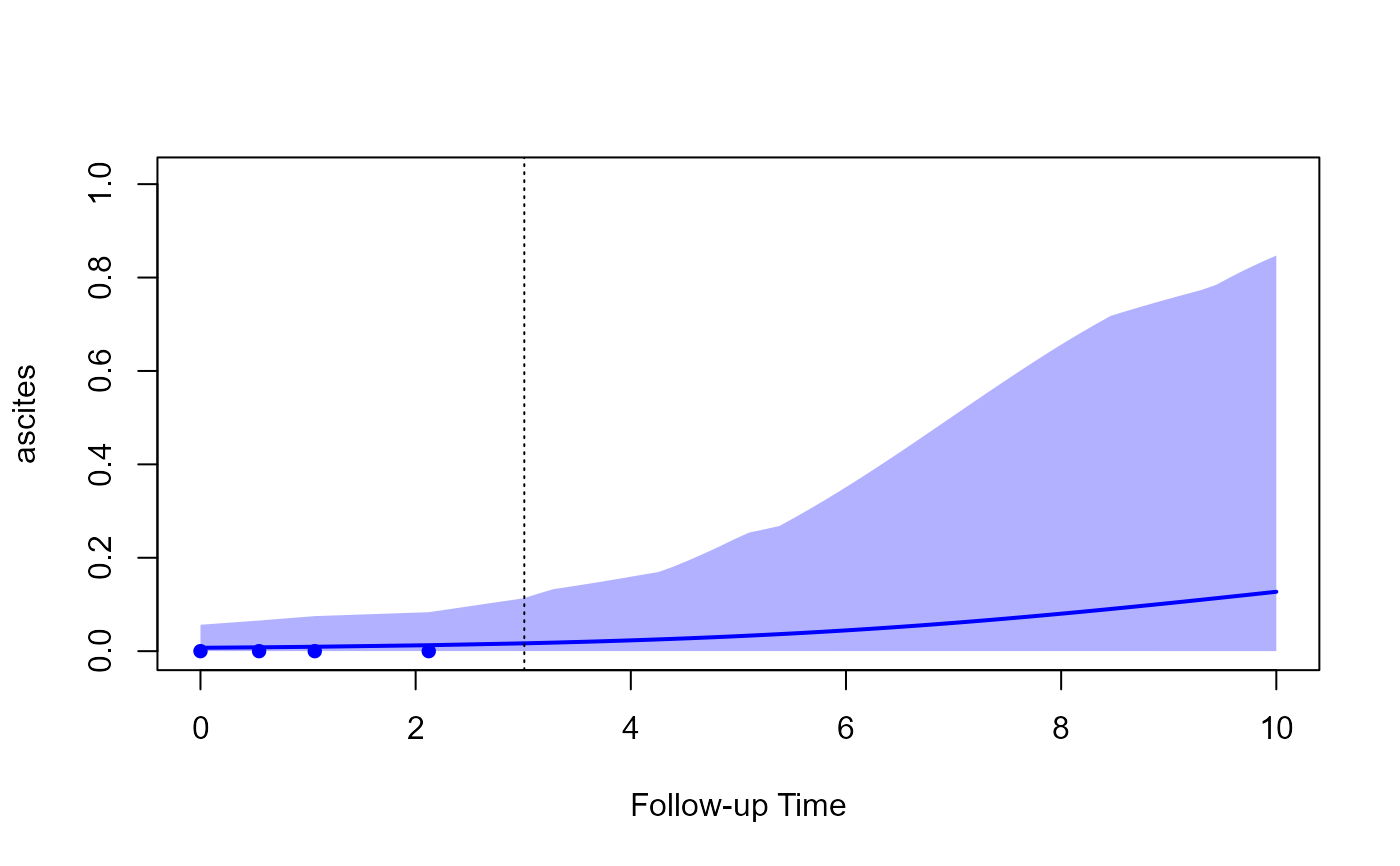
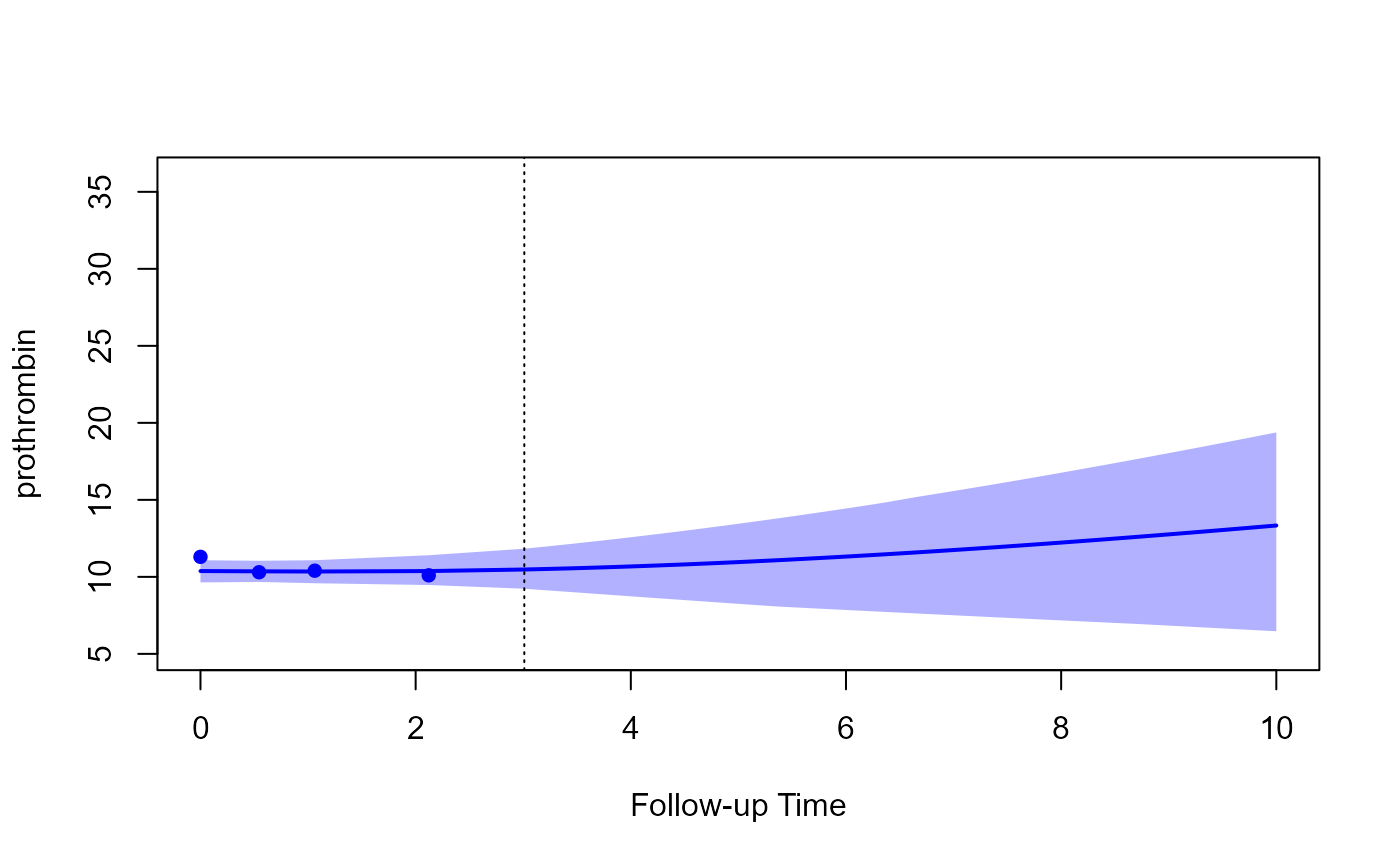
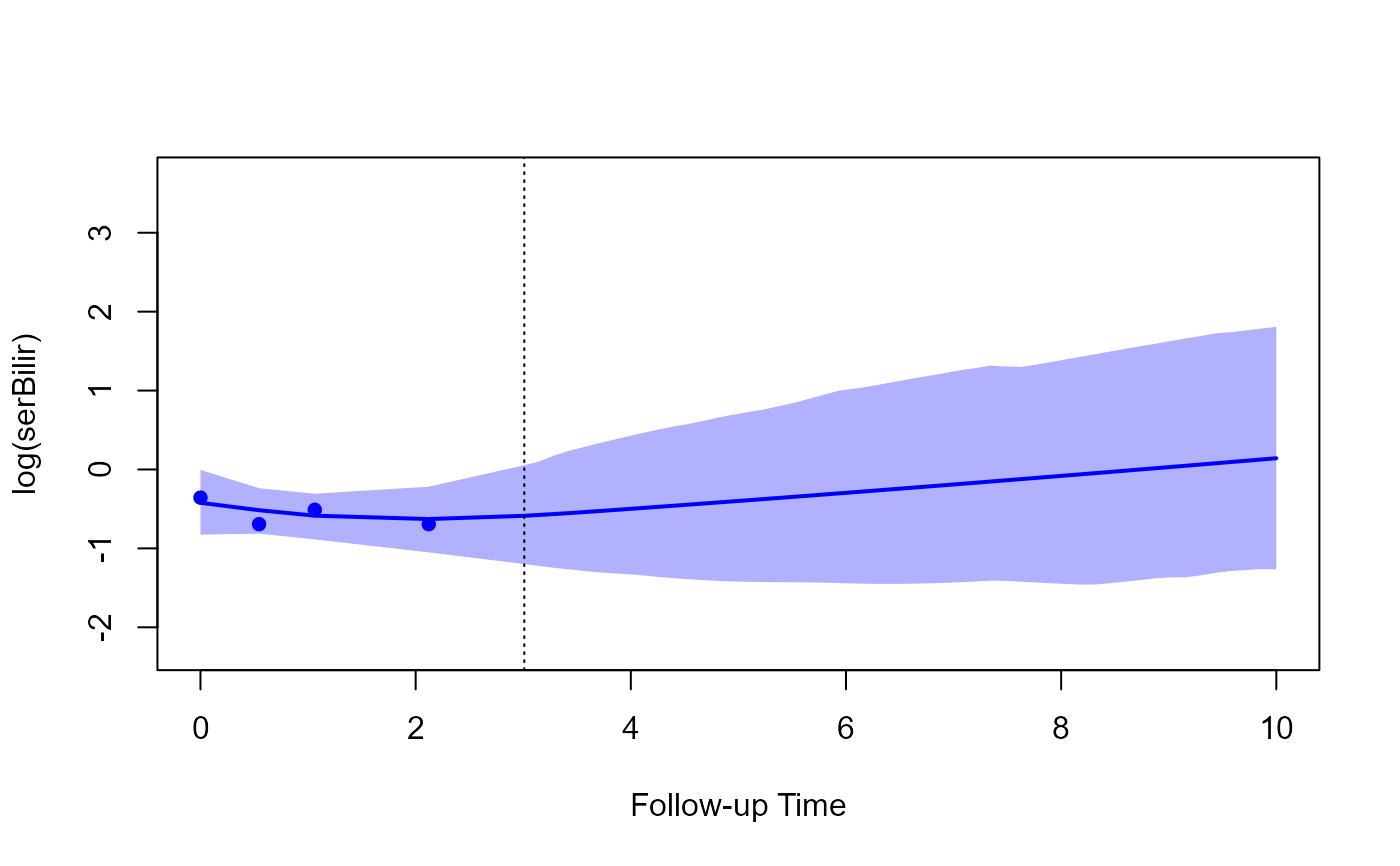
# predictions for the longitudinal outcomes using newdata
predLong1 <- predict(jointFit, newdata = ND, return_newdata = TRUE)

# predictions for the longitudinal outcomes at future time points
# from year 3 to 10
predLong2 <- predict(jointFit, newdata = ND,
                     times = seq(t0, 10, length.out = 51),
                     return_newdata = TRUE)

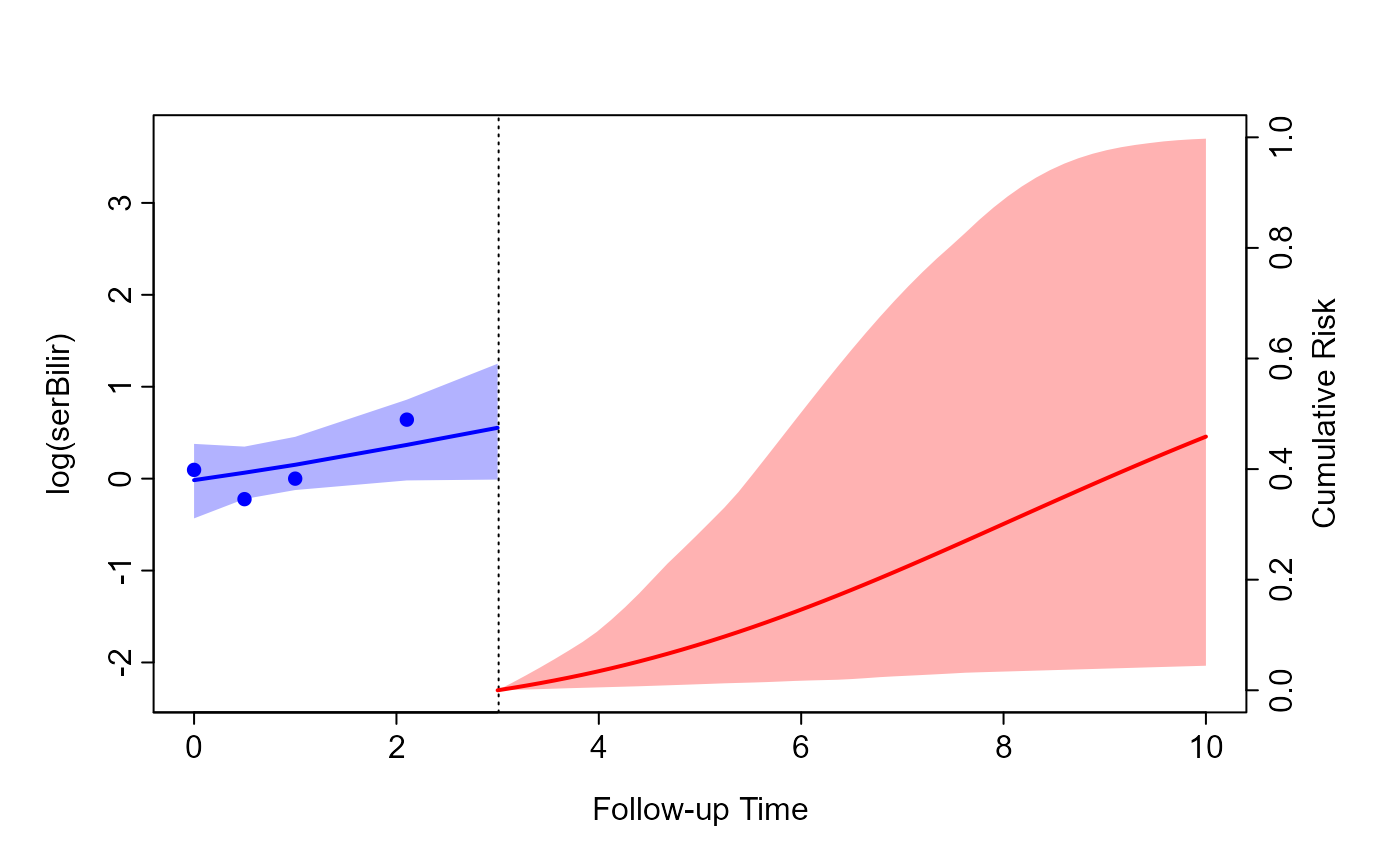
# predictions for the event outcome at future time points
# from year 3 to 10
predSurv <- predict(jointFit, newdata = ND, process = "event",
                    times = seq(t0, 10, length.out = 51),
                    return_newdata = TRUE)

plot(predLong1)

# for subject 25, outcomes in reverse order
plot(predLong2, outcomes = 3:1, subject = 25)




# prediction for the event outcome
plot(predSurv)


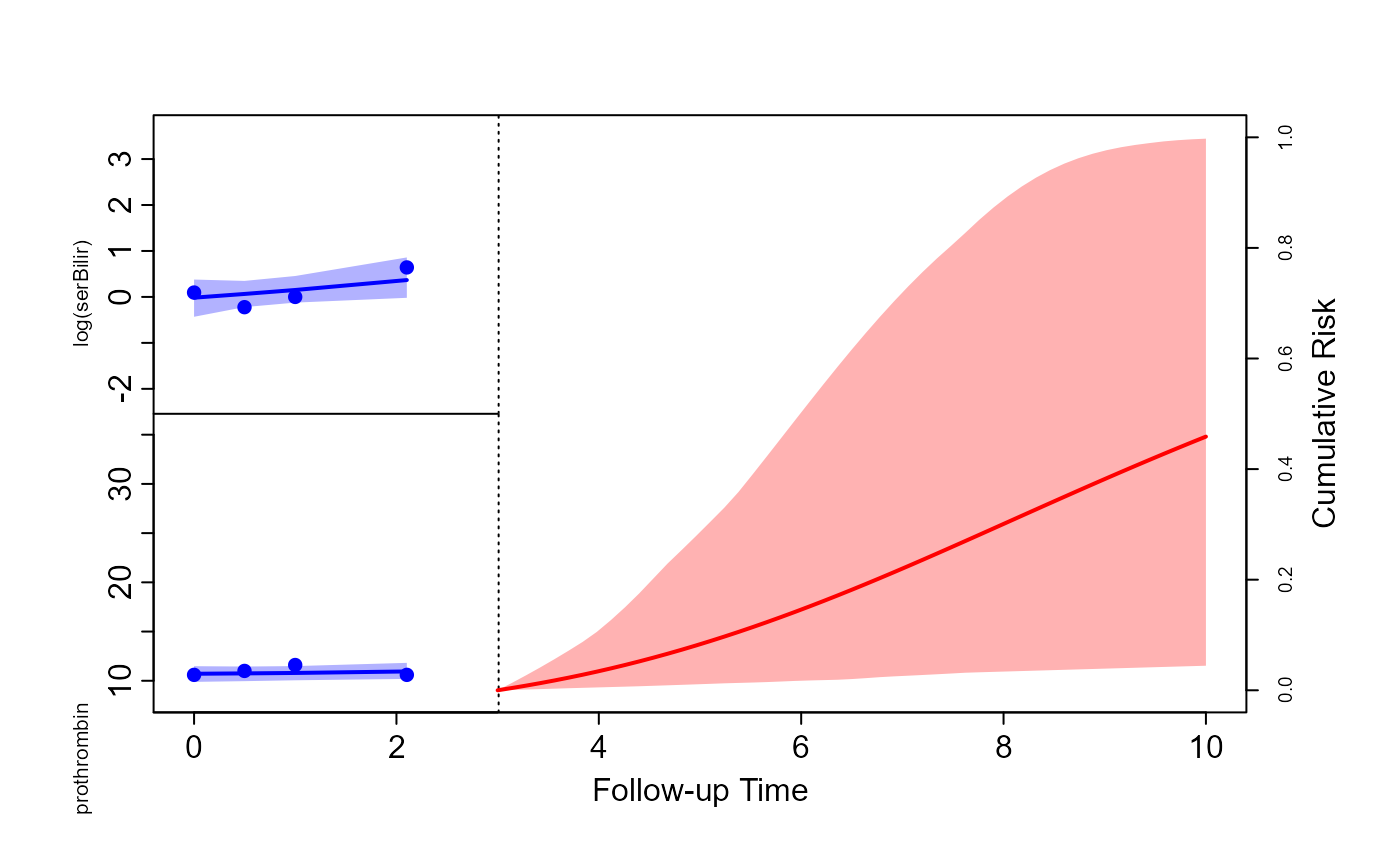
# combined into one plot, the first longitudinal outcome and cumulative risk
plot(predLong2, predSurv, outcomes = 1)


# the first two longitudinal outcomes
plot(predLong1, predSurv, outcomes = 1:2)


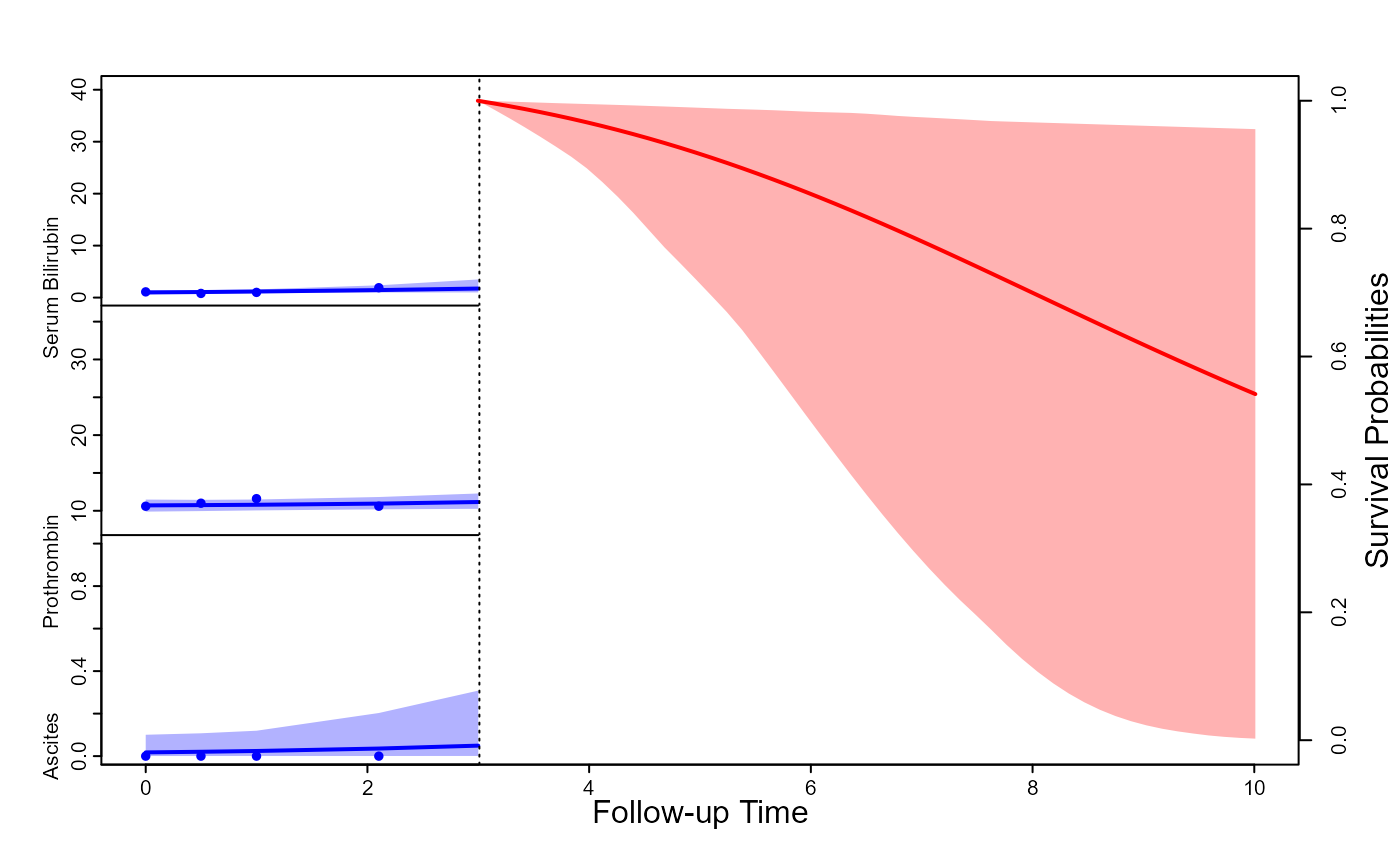
# all three longitudinal outcomes, we display survival probabilities instead
# of cumulative risk, and we transform serum bilirubin to the original scale
plot(predLong2, predSurv, outcomes = 1:3, fun_event = function (x) 1 - x,
     fun_long = list(exp, identity, identity),
     ylab_event = "Survival Probabilities",
     ylab_long = c("Serum Bilirubin", "Prothrombin", "Ascites"),
     pos_ylab_long = c(1.9, 1.9, 0.08))

# }