Causal Effects

Causal Effects from Joint Models

We will illustrate the calculation of causal effects from joint models using the PBC dataset for the longitudinal outcome serBilir and the composite event transplantation or death. We start by fitting a joint model to the data. In the longitudinal submodel, we specify nonlinear subject-specific trajectories using natural cubic splines. In the fixed-effects part, we also include the treatment effect and its interaction with time. In the survival submodel, we only include the treatment effect.

pbc2.id$status2 <- as.numeric(pbc2.id$status != "alive")
lmeFit <- lme(log(serBilir) ~ ns(year, 3, B = c(0, 14.4)) * drug, 
                   data = pbc2, random = ~ ns(year, 3, B = c(0, 14.4)) | id,
                   control = lmeControl(opt = "optim"))
CoxFit <- coxph(Surv(years, status2) ~ drug, data = pbc2.id)
jmFit <- jm(CoxFit, lmeFit, time_var = "year")
summary(jmFit)
#> 
#> Call:
#> jm(Surv_object = CoxFit, Mixed_objects = lmeFit, time_var = "year")
#> 
#> Data Descriptives:
#> Number of Groups: 312        Number of events: 169 (54.2%)
#> Number of Observations:
#>   log(serBilir): 1945
#> 
#>                  DIC     WAIC      LPML
#> marginal    4217.836 4527.502 -2937.053
#> conditional 6503.006 6206.639 -3454.250
#> 
#> Random-effects covariance matrix:
#>                                                                       
#>                    StdDev   Corr                                      
#> (Intr)             0.9958 (Intr) n(,3,B=c(0,14.4))1 n(,3,B=c(0,14.4))2
#> n(,3,B=c(0,14.4))1 1.5005 0.2219                                      
#> n(,3,B=c(0,14.4))2 1.6970 0.4318 0.7505                               
#> n(,3,B=c(0,14.4))3 1.8995 0.4247 0.2076             0.6798            
#> 
#> Survival Outcome:
#>                         Mean  StDev    2.5%  97.5%      P   Rhat
#> drugD-penicil        -0.0138 0.2061 -0.4079 0.3859 0.9533 1.0037
#> value(log(serBilir))  1.3001 0.0881  1.1354 1.4741 0.0000 1.0109
#> 
#> Longitudinal Outcome: log(serBilir) (family = gaussian, link = identity)
#>                        Mean  StDev    2.5%  97.5%      P   Rhat
#> (Intercept)          0.5863 0.0808  0.4309 0.7430 0.0000 1.0007
#> ns(,3,B=c(0,14.4))1  1.1251 0.1719  0.7905 1.4659 0.0000 1.0058
#> ns(,3,B=c(0,14.4))2  2.1954 0.2329  1.7749 2.6913 0.0000 1.0201
#> ns(,3,B=c(0,14.4))3  2.4177 0.3416  1.8350 3.1714 0.0000 1.0342
#> drugD-penicil       -0.1061 0.1163 -0.3386 0.1217 0.3633 1.0017
#> n(,3,B=c(0,14.4))1:  0.1869 0.2369 -0.2802 0.6490 0.4218 1.0055
#> n(,3,B=c(0,14.4))2: -0.4776 0.3224 -1.1454 0.1111 0.1211 1.0175
#> n(,3,B=c(0,14.4))3: -0.6994 0.4770 -1.7031 0.1481 0.1233 1.0384
#> sigma                0.2894 0.0065  0.2776 0.3027 0.0000 1.0061
#> 
#> MCMC summary:
#> chains: 3 
#> iterations per chain: 3500 
#> burn-in per chain: 500 
#> thinning: 1 
#> time: 21 sec

The coefficient for drugD-penicil for the survival outcome in the output produced by the summary() method denotes the residual/direct effect of treatment on the risk of the composite event. It does not include the effect of treatment that follows via the serum bilirubin pathway.

We will illustrate the calculation of causal risk differences for the group of patients that have the same distribution of serum bilirubin values as Patient 2:

xyplot(log(serBilir) ~ year, data = pbc2, subset = id == 2, type = "b",
       xlab = "Follow-up time (years)", ylab = "log{serum bilirubin (mg/dL)}",
       main = "Patient 2")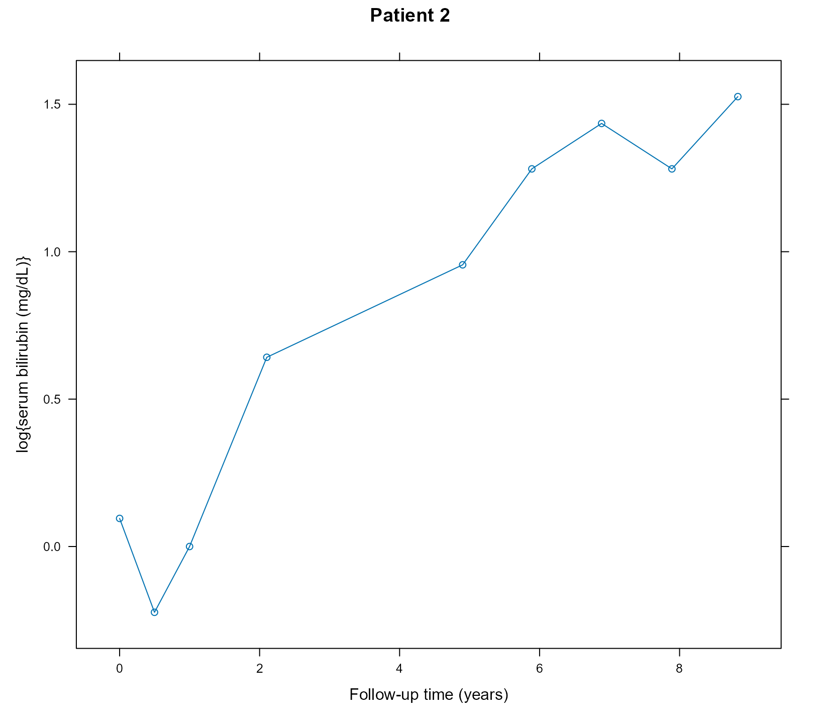

We calculate the risk difference for the composite event between the active treatment D-penicillamine and placebo at the horizon time t_horiz = 6 using the longitudinal data up to year t0 = 4. To achieve this, we create a dataset with this patient’s data. This patient received the active treatment D-penicillamine; hence, we also create a version of her data with the drug variable set to placebo:

t0 <- 4
t_horiz <- 6
dataP2_Dpenici <- pbc2[pbc2$id == 2 & pbc2$year <= t0, ]
dataP2_Dpenici$years <- t0
dataP2_Dpenici$status2 <- 0

dataP2_placebo <- dataP2_Dpenici
dataP2_placebo$drug <- factor("placebo", levels = levels(pbc2$drug))

Note that in the dataP2_placebo dataset, we need to specify that drug is a factor with two levels. We also specify that the last time point we know the patient was still event-free was t0.

We estimate the cumulative risk for the composite event at t_horiz under the active treatment arm using the predict() method:

Pr1 <- predict(jmFit, newdata = dataP2_Dpenici, process = "event", 
               times = t_horiz, return_mcmc = TRUE)

We have set the argument return_mcmc to TRUE to enable the calculation of a credible interval that accounts for the MCMC uncertainty. We produce the same estimate under the placebo arm:

Pr0 <- predict(jmFit, newdata = dataP2_placebo, process = "event", 
               times = t_horiz, return_mcmc = TRUE)

The estimated risk difference and its 95% credible interval are calculated by the corresponding elements of the Pr1 and Pr0 objects, i.e.,

# estimate 
Pr1$pred[2L] - Pr0$pred[2L]
#> [1] 0.002916423

# MCMC variability
quantile(Pr1$mcmc[2L, ] - Pr0$mcmc[2L, ], probs = c(0.025, 0.975))
#>       2.5%      97.5% 
#> -0.1790905  0.1952539

Time-varying treatments

An extended example with time-varying treatments / intermediate events that showcases a calculation of the variance of the causal effects that includes the sampling variability is available here.

Dimitris Rizopoulos

2025-08-23

Causal Effects from Joint Models

Time-varying treatments