Recurrent Events
Pedro Miranda-Afonso
2026-02-02
Source:vignettes/Recurring_Events.Rmd
Recurring_Events.RmdJoint Models with Recurrent events
Introduction
JMbayes2 also provides the capability to fit joint models with a recurrent event process, possibly combined with a terminating event. Recurrent events are correlated events that may occur more than once over the follow-up period for a given subject. For a real-data application of this framework, see Miranda-Afonso et al. (2025).
Our current implementation allows for multiple longitudinal markers with different distributions and various functional forms to link these markers with the risk of recurrent and terminal events. Furthermore, it enables the risk intervals to be defined in terms of the gap or calendar timescales. The two timescales use a different zero-time reference. The calendar uses the study entry, while the gap uses the end of the previous event (Figure 1). Gap assumes a renewal after each event and resets the time to zero.
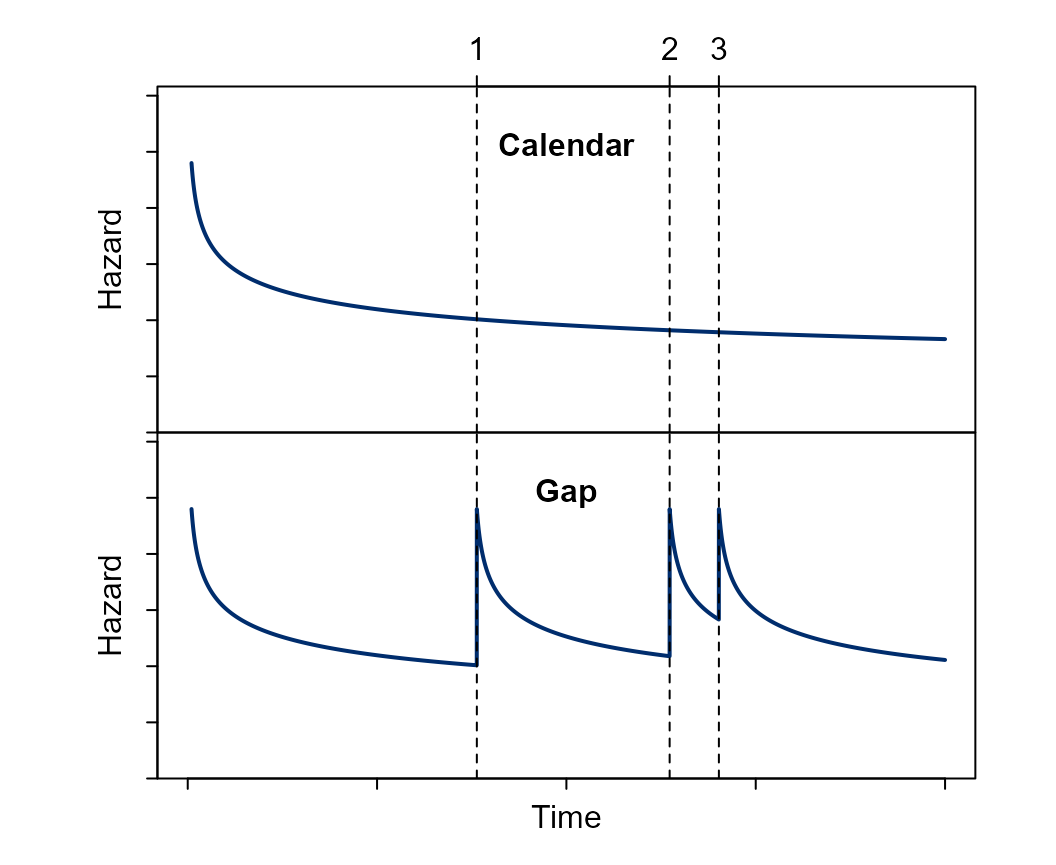
Figure 1 Visual representation of an hazard function under the gap or calendar timescale. During the follow-up, the subject experienced three events.
The model also accommodates discontinuous risk intervals, i.e., periods in which the subject is not at risk of experiencing the recurring event (Figure 2). For example, while a patient is in the hospital, they are not at risk of being hospitalized again.
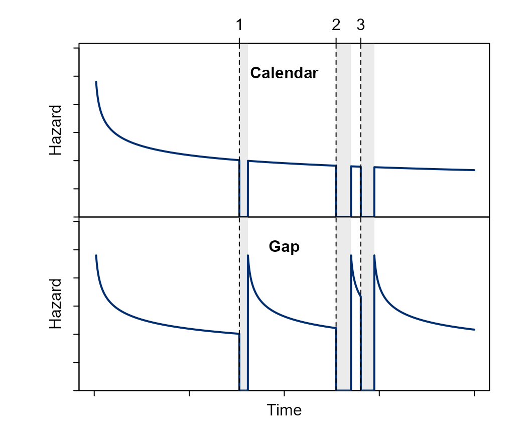
Figure 2 Visual representation of an hazard function under the gap or calendar timescale, while accounting for non-risk periods (gray areas). During the follow-up, the subject experienced three events.
A joint model with p normally distributed longitudinal markers, a terminal event process, and a recurrent event process can be described as follows:
\small{ \begin{cases} y_{1_i}(t)= x_{1_i}(t)^\top \beta_1 + z_{1_i}(t)^\top b_{1_i} + \varepsilon_1(t) = \eta_{1_i}(t) + \varepsilon_1(t) & \text{Longitudinal marker 1,}\\ \vdots \\ y_{p_i}(t)= x_{p_i}(t)^\top \beta_p + z_{p_i}(t)^\top b_{p_i} + \varepsilon_p(t) = \eta_{p_i}(t) + \varepsilon_p(t) & \text{Longitudinal marker p,}\\ h_{T_i}(t)= h_{T_0}(t)\exp \left \{ w_{T_i}(t)^\top \gamma_T + \mathcal{f}_{T_1}\left\{\eta_{1_i}(t)\right\} \alpha_{T_1} + \dots + \mathcal{f}_{T_p}\left\{\eta_{p_i}(t)\right\} \alpha_{T_p} + b_{F_i} \alpha_{F} \right\} & \text{Terminal event,}\\ h_{R_i}(t)= h_{R_0}(t)\exp\left\{ w_{R_i}(t)^\top \gamma_R + \mathcal{f}_{R_1}\left\{\eta_{2_i}(t)\right\} \alpha_{R_1} + \dots + \mathcal{f}_{R_p}\left\{\eta_{p_i}(t)\right\} \alpha_{R_p} + b_{F_i} \right\} & \text{Recurrent event,}\\ \end{cases} }
\begin{pmatrix} b_{1_i} \\ \vdots \\ b_{p_i} \\ b_{F_i}\end{pmatrix} \sim \mathcal{N} \left(0, \begin{pmatrix}D & 0 \\ & \sigma^2_F\end{pmatrix}\right), \qquad \varepsilon(t) \sim N \left(0, \sigma^2\right),
where i = 1, \ldots, n. We specify linear mixed-effects models for the longitudinal outcomes, and for the terminal and recurrence processes, we use proportional hazard models. The longitudinal and event time processes are linked via a latent structure of random effects, highlighted by the same color in the equations above. The terms \mathcal{f}_{R_j}\left\{\eta_{j_i}(t)\right\} and \mathcal{f}_{R_j}\left\{\eta_{j_i}(t)\right\} describe the functional forms that link the longitudinal marker j with the risk of the recurrent and terminal events, respectively. The frailty b_{F_i} is a random effect that accounts for the correlations in the recurrent events. The coefficient \alpha_{F} quantifies the strength of the association between the terminal and recurrent event processes. For notational simplicity, in the formulation presented above, we have shown normally distributed longitudinal outcomes; however, JMbayes2 provides the option to consider longitudinal outcomes with different distributions.
Example
Data
We simulate data from a joint model with three outcomes: one longitudinal outcome, one terminal failure time, and one recurrent failure time. We assume that the underlying value of the longitudinal outcome is associated with both risk models and use the gap timescale. The reader can easily extend this example to accommodate multiple longitudinal markers with other forms of association, including competing risks, considering only the recurrent events process, or using a different timescale.
gen_data <- function(){
  n <- 500 # desired number of subjects
  n_i <- 15  # number of (planned) measurements per subject
  tmax <- 7 # maximum follow-up time (type I censoring)
  scale <- "gap" # hazard timescale
  ##############################################################################
  n_scl <- 1.5
  n_target <- n
  n <- n * n_scl
  # longitudinal outcome 1/2
  ## param true values
  betas <- c("Intercept" = 6.94, "Time1" = 1.30, "Time2" = 1.84, "Time3" = 1.82)
  sigma_y <- 0.6 # measurement error sd
  D <- matrix(0, 4, 4)
  D[lower.tri(D, TRUE)] <- c(0.71, 0.33, 0.07, 1.26, 2.68, 3.81, 4.35, 7.62, 5.4, 8)
  D <- D + t(D)
  diag(D) <- diag(D) * 0.5
  b <- MASS::mvrnorm(n, rep(0, nrow(D)), D)
  Bkn <- c(0, 7)
  kn <- c(1, 3)
  remove(D)
  ##############################################################################
  # terminal outcome
  ## param true values
  gammas_t <- c("(Intercept)" = -9, "Group" = 0.5, "Age" = 0.05) # phi = exp(Intercept)
  sigma_t <- 2
  alpha_t <- 0.5 # association biomarker
  alphaF <- 0.25 # association frailty
  sigmaF <- 0.25 # frailty SD
  frailty <- rnorm(n, mean = 0, sd = sigmaF)
  ## terminal data
  group <- rep(0:1, each = n/2)
  age <- runif(n, 30, 70)
  W_t <- cbind("(Intercept)" = 1, "Group" = group, "Age" = age)
  eta_t <- as.vector(W_t %*% gammas_t + alphaF * frailty)
  invS_t <- function(t, u, i) {
    h <- function(s) {
      NS <- splines::ns(s, knots = kn, Boundary.knots = Bkn)
      X <- cbind(1, NS)
      Z <- cbind(1, NS)
      eta_y <- as.vector(X %*% betas + rowSums(Z * b[rep(i, nrow(Z)), ]))
      exp(log(sigma_t) + (sigma_t - 1) * log(s) + eta_t[i] + eta_y * alpha_t)
    }
    integrate(h, lower = 0, upper = t)$value + log(u)
  }
  u_t <- runif(n)
  ter_times <- numeric(n)
  for(i in seq_len(n)) {
    root <- try(uniroot(invS_t, interval = c(1e-05, 250), # arbitrary upper limit
                        u = u_t[i], i = i)$root, TRUE)
    ter_times[i] <- if (!inherits(root, "try-error")) root else NA
  }
  ter_na <- !is.na(ter_times)
  if(sum(ter_na) < n_target) stop("Not enough patients. Increase 'n_scl'.")
  rmv_ids <- sample(which(ter_na), sum(ter_na) - n_target)
  ter_na[rmv_ids] <- FALSE # remove the excess of subjects
  ter <- data.frame(id    = seq_len(n)[ter_na],
                    tstop = ter_times[ter_na],
                    group = group[ter_na],
                    age   = age[ter_na])
  frailty <- frailty[ter_na]
  b <- b[ter_na, , drop = FALSE]
  cens_times <- tmax
  ter$status <- as.numeric(ter$tstop <= cens_times) # event indicator
  ter$tstop <- pmin(ter$tstop, cens_times) # add censoring time
  remove(gammas_t, sigma_t, group, W_t, eta_t, alpha_t, invS_t, u_t, i, root,
         n_target, rmv_ids, ter_times, cens_times, n, alphaF, age, ter_na,
         sigmaF)
  ##############################################################################
  # recurring outcome
  ## param true values
  gammas_r <- c("(Intercept)" = -9+3, "Group" = 0.5, "Age" = 0.05) # phi = exp(Intercept)
  sigma_r <- 2
  alpha_r <- 0.5 # association biomarker
  ## recurring data
  W_r <- cbind("(Intercept)" = 1, "Group" = ter$group, "Age" = ter$age)
  eta_r <- as.vector(W_r %*% gammas_r + frailty)
  if(scale == "gap") {
    invS_r <- function(t, u, i, tstart) {
      h <- function(s) {
        NS <- splines::ns(s + tstart, knots = kn, Boundary.knots = Bkn)
        X <- cbind(1, NS)
        Z <- cbind(1, NS)
        eta_y <- as.vector(X %*% betas + rowSums(Z * b[rep(i, nrow(Z)), ]))
        exp(log(sigma_r) + (sigma_r - 1) * log(s) + eta_r[i] + eta_y * alpha_r)
      }
      integrate(h, lower = 0, upper = t)$value + log(u)
    }
  } else if(scale == "calendar") {
    invS_r <- function(t, u, i, tstart) {
      h <- function(s) {
        NS <- splines::ns(s + tstart, knots = kn, Boundary.knots = Bkn)
        X <- cbind(1, NS)
        Z <- cbind(1, NS)
        eta_y <- as.vector(X %*% betas + rowSums(Z * b[rep(i, nrow(Z)), ]))
        exp(log(sigma_r) + (sigma_r - 1) * log(s + tstart) + eta_r[i] + eta_y * alpha_r)
      }
      integrate(h, lower = 0, upper = t)$value + log(u)
    }
  }
  stop_times <- start_times <- id_times <- list()
  j <- 1
  for(i in seq_along(ter$id)) {
    tstart <- 0
    while(!is.na(tstart) & tstart < ter$tstop[i]) {
      u_r <- runif(1)
      root <- try(uniroot(invS_r, interval = c(1e-05, 250), # arbitrary upper limit
                          u = u_r, i = i, tstart = tstart)$root, TRUE)
      tstop <- if(!inherits(root, "try-error")) root else NA
      start_times[[j]] <- tstart
      stop_times[[j]] <- tstart + tstop
      dur <- runif(1, 0, 0.1) # recurrent event duration
      tstart <- tstart + tstop + dur
      id_times[[j]] <- ter$id[i]
      j <- j + 1
    }
  }
  rec <- data.frame(id     = unlist(id_times),
                    tstart = unlist(start_times),
                    tstop  = unlist(stop_times))
  rec$id  <- match(rec$id, unique(rec$id)) # rename IDs
  rec$group <- ter$group[rec$id]
  rec$age <- ter$age[rec$id]
  rec$Stime <- ter$tstop[rec$id]
  rec$status <- as.numeric(!is.na(rec$tstop) & rec$tstop < rec$Stime)  # event indicator
  rec$tstop <- pmin(rec$tstop, rec$Stime, na.rm = TRUE) # add cens time
  rec$Stime <- NULL
  ter$id <- seq_along(ter$id)
  remove(gammas_r, sigma_r, W_r, eta_r, alpha_r, invS_r, stop_times, start_times,
         id_times, dur, j, i, tstart, u_r, root, tstop)
  ##############################################################################
  # longitudinal outcome 2/2
  long <- data.frame(id   = rep(ter$id, each = n_i),
                     time = c(replicate(length(ter$id), c(0, sort(runif(n_i - 1, 1, tmax))))))
  X <- model.matrix(~ 1 + splines::ns(time, knots = kn, Boundary.knots = Bkn),
                    data = long)
  Z <- model.matrix(~ 1 + splines::ns(time, knots = kn, Boundary.knots = Bkn),
                    data = long)
  eta_y <- as.vector(X %*% betas + rowSums(Z * b[long$id, ]))
  long$y <- rnorm(length(eta_y), eta_y, sigma_y)
  long_cens <- long$time <= rep(ter$tstop, times = rle(long$id)$lengths)
  long <- long[long_cens, , drop = FALSE] # drop censored encounters
  remove(kn, Bkn, X, betas, Z, b, eta_y, sigma_y, n_i, tmax, long_cens, scale)
  ##############################################################################
  # return
  list(long = long, ter = ter, rec = rec)
}
set.seed(2022); fake_data <- gen_data()
term_data <- fake_data$ter # terminal event data
recu_data <- fake_data$rec # recurrent events data
lme_data <- fake_data$long # longitudial marker data
We now have three data frames, each one corresponding to a different
outcome. To fit the joint model, the user must organize the failure-time
data in the counting process formulation by combining the data for the
terminal and recurrent events. Then, a strata variable is used to
distinguish between the two processes. To facilitate this, we provide in
the package the rc_setup() function:
cox_data <- rc_setup(rc_data = recu_data, trm_data = term_data,
                     idVar = "id", statusVar = "status",
                     startVar = "tstart", stopVar = "tstop",
                     trm_censLevel = 0,
                     nameStrata = "strata", nameStatus = "status")
Each subject has as many rows in the new data frame as the number of
their recurrent risk periods plus one for the terminal event. The data
frame follows the counting process formulation with the risk intervals
delimited by start and stop variables. The
strata variable denotes the type of event, 1
if recurrent, or 2 terminal. The status equals
1 if the subject had an event and 0 otherwise.
As shown below and in Figure 3, subject 1 experienced seven recurrent
events during the follow-up; the terminal event censored the eighth
recurrent event.
cox_data[cox_data$id == 1, c("id", "tstart", "tstop", "status", "strata")]
#>   id    tstart     tstop status strata
#> 1  1 0.0000000 0.3756627      1      R
#> 2  1 0.4275324 0.7832841      1      R
#> 3  1 0.8724938 1.0863887      1      R
#> 4  1 1.1212953 1.8741434      1      R
#> 5  1 1.9372355 2.7843451      1      R
#> 6  1 2.7906559 3.4618622      1      R
#> 7  1 3.5166929 3.5830169      1      R
#> 8  1 3.6251219 4.0375415      0      R
#> 9  1 0.0000000 4.0375415      1     T1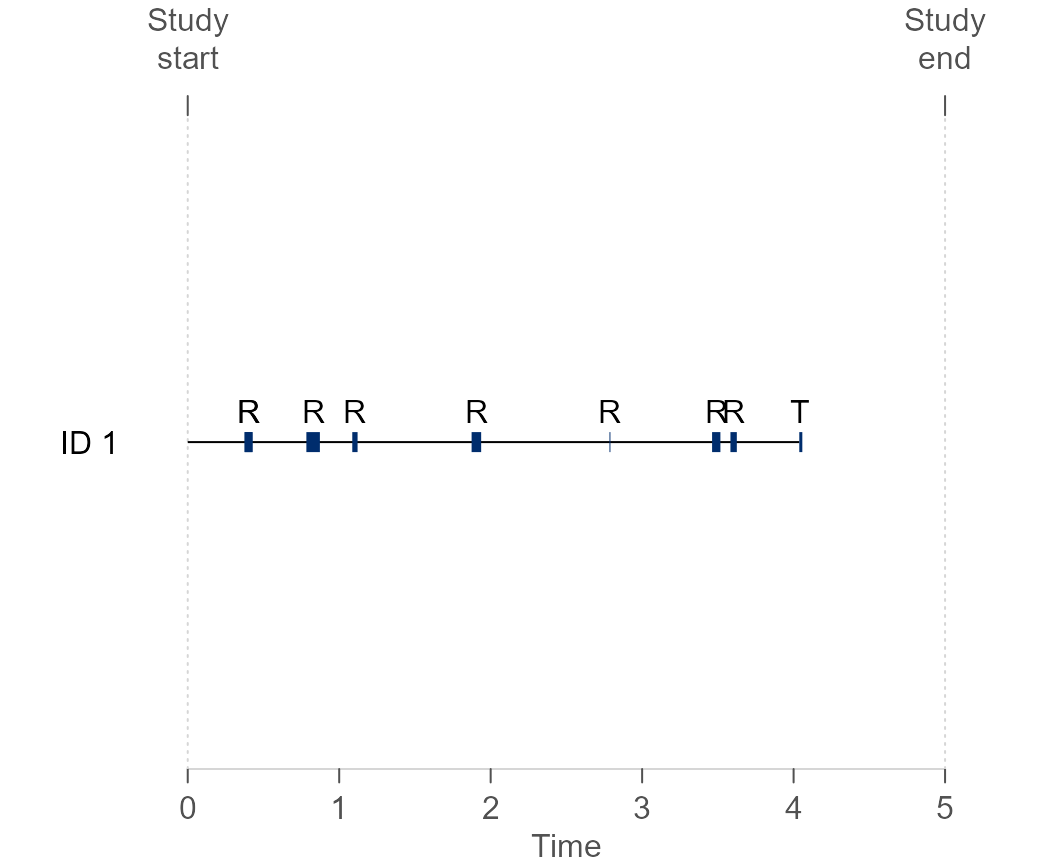
Figure 3 Visual representation of the failure-time data during the follow-up for subject 1. The horizontal black line denotes risk periods, while the blue line denotes non-risk periods. ‘R’ and ‘T’ represent a recurrent and terminal event, respectively.
Fitting the model
The user then needs to use the nlme::lme() function
first to fit the linear mixed model that describes the longitudinal
outcome,
lme_fit <- lme(y ~ ns(time, k =  c(1, 3), B = c(0, 7)),
               random = list(id = pdDiag(form = ~ ns(time, k = c(1, 3),
                                                       B = c(0, 7)))),
               data = lme_data,
               control = lmeControl(opt = "optim", niterEM = 45))
Then, we use the survival::coxph() function to fit a
stratified Cox model using the transformed data,
These models are then provided as arguments in the jm()
function. The user specifies the desired functional forms for the mixed
model in each relative-risk model. And with the recurrent
argument specifying the desired timescale,
jm_fit <- jm(cox_fit, lme_fit, time_var = "time", recurrent = "gap",
             functional_forms =  ~ value(y):strata)

summary(jm_fit)
#>
#> Call:
#> JMbayes2::jm(Surv_object = cox_fit, Mixed_objects = lme_fit,
#>     time_var = "time", recurrent = "gap", functional_forms = ~value(y):strata)
#>
#> Data Descriptives:
#> Number of Groups: 500        Number of events: 2250 (81.6%)
#> Number of Observations:
#>   y: 3075
#>
#>                  DIC     WAIC       LPML
#> marginal    13149.97 12983.05  -6736.434
#> conditional 19832.17 19095.66 -10201.566
#>
#> Random-effects covariance matrix:
#>
#>                        StdDev   Corr
#> (Intr)                 0.7423 (Intr) n(,k=c(1,3),B=c(0,7))1
#> n(,k=c(1,3),B=c(0,7))1 2.0832
#> n(,k=c(1,3),B=c(0,7))2 1.4450
#> n(,k=c(1,3),B=c(0,7))3 1.7567
#>
#>
#> (Intr)                 n(,k=c(1,3),B=c(0,7))2
#> n(,k=c(1,3),B=c(0,7))1
#> n(,k=c(1,3),B=c(0,7))2
#> n(,k=c(1,3),B=c(0,7))3
#>
#> Frailty standard deviation:
#>                 Mean   2.5%  97.5%
#> sigma_frailty 0.1928 0.0212 0.3105
#>
#> Survival Outcome:
#>                             Mean  StDev    2.5%  97.5%      P   Rhat
#> group:strata(strata)R     0.4638 0.0826  0.3032 0.6233 0.0000 1.0022
#> group:strata(strata)T1    0.4348 0.1071  0.2215 0.6346 0.0000 1.0204
#> age:strata(strata)R       0.0497 0.0029  0.0442 0.0555 0.0000 1.0395
#> age:strata(strata)T1      0.0475 0.0048  0.0383 0.0570 0.0000 1.2322
#> value(y):strataR          0.5071 0.0275  0.4563 0.5605 0.0000 1.0678
#> value(y):strataT1         0.4983 0.0402  0.4222 0.5762 0.0000 1.5801
#> frailty:strata(strata)T1 -0.6146 1.1373 -3.0913 2.2689 0.3878 1.1494
#>
#> Longitudinal Outcome: y (family = gaussian, link = identity)
#>                           Mean  StDev    2.5%  97.5%      P   Rhat
#> (Intercept)             6.9873 0.0427  6.9034 7.0701 0.0000 1.0228
#> n(,k=c(1,3),B=c(0,7))1  1.3662 0.1472  1.0788 1.6537 0.0000 1.0120
#> n(,k=c(1,3),B=c(0,7))2  0.6188 0.1477  0.3321 0.9173 0.0000 1.3360
#> n(,k=c(1,3),B=c(0,7))3 -0.1523 0.2027 -0.5384 0.2605 0.4333 1.2847
#> sigma                   0.6159 0.0100  0.5960 0.6356 0.0000 1.0121
#>
#> MCMC summary:
#> chains: 3
#> iterations per chain: 3500
#> burn-in per chain: 500
#> thinning: 1
#> time: 1.7 min
One can find the association parameters between the underlying value
of the longitudinal outcome and the recurrent and terminating event
processes in the summary output as value(y):strataRec
(\alpha_{R_1}) and
value(y):strataTer (\alpha_{T_1}), respectively. \exp\{\alpha_{R_1}\} denotes the relative
increase in the risk of the next recurrent event at time t that results from one unit increase in
\eta_{1_i}(t) since the end of the
previous event1. The association parameter for the frailty
term in the terminal risk model, \alpha_{F}, is identified in the output as
frailty. The sigma_frailty refers to the
frailty standard deviation, \sigma_F.