Various Methods for Functions from the coda Package
coda_methods.RdMethods for an object of class "jm" for diagnostic functions.
Usage
traceplot(object, ...)

# S3 method for class 'jm'
traceplot(object,
  parm = c("all", "betas", "sigmas", "D", "bs_gammas",
           "tau_bs_gammas", "gammas", "alphas"), ...)

ggtraceplot(object, ...)

# S3 method for class 'jm'
ggtraceplot(object,
  parm = c("all", "betas", "sigmas", "D", "bs_gammas",
           "tau_bs_gammas", "gammas", "alphas"),
  linewidth = 1, alpha = 0.8,
  theme = c('standard', 'catalog', 'metro',
                'pastel', 'beach', 'moonlight', 'goo', 'sunset', 'custom'),
  grid = FALSE, gridrows = 3, gridcols = 1, custom_theme = NULL, ...)

gelman_diag(object, ...)

# S3 method for class 'jm'
gelman_diag(object,
  parm = c("all", "betas", "sigmas", "D", "bs_gammas",
           "tau_bs_gammas", "gammas", "alphas"), ...)

densplot(object, ...)

# S3 method for class 'jm'
densplot(object,
  parm = c("all", "betas", "sigmas", "D", "bs_gammas",
           "tau_bs_gammas", "gammas", "alphas"), ...)

ggdensityplot(object, ...)

# S3 method for class 'jm'
ggdensityplot(object,
  parm = c("all", "betas", "sigmas", "D", "bs_gammas",
           "tau_bs_gammas", "gammas", "alphas"),
  linewidth = 1, alpha = 0.6,
  theme = c('standard', 'catalog', 'metro', 'pastel',
                'beach', 'moonlight', 'goo', 'sunset', 'custom'),
  grid = FALSE, gridrows = 3, gridcols = 1, custom_theme = NULL, ...)

cumuplot(object, ...)

# S3 method for class 'jm'
cumuplot(object,
  parm = c("all", "betas", "sigmas", "D", "bs_gammas",
           "tau_bs_gammas", "gammas", "alphas"), ...)
Arguments
- object
an object inheriting from class
"jm".- parm
a character string specifying which parameters of the joint model to plot. Possible options are
'all','betas','alphas','sigmas','D','bs_gammas','tau_bs_gammas', or'gammas'.- linewidth
the width of the traceplot line in mm. Defaults to 1.
- alpha
the opacity level of the traceplot line. Defaults to 0.8.
- theme
a character string specifying the color theme to be used. Possible options are
'standard','catalog','metro','pastel','beach','moonlight','goo', or'sunset'. Note that this option supports fitted objects with three chains. If the object was fitted using a different number of chains then the colors are either automatically chosen, or can be specified by the user via the argumentcustom_theme.- grid
logical; defaults to
FALSE. IfTRUE, the plots are returned in grids split over multiple pages. For more details see the documentation forgridExtra::marrangeGrob().- gridrows
number of rows per page for the grid. Only relevant when using
grid = TRUE. Defaults to 3.- gridcols
number of columns per page for the grid. Only relevant when using
grid = TRUE. Defaults to 1.- custom_theme
A named character vector with elements equal to the number of chains (
n_chains). The name of each element should be the number corresponding to the respective chain. Defaults toNULL.- ...
further arguments passed to the corresponding function from the coda package.
Value
traceplot()Plots the evolution of the estimated parameter vs. iterations in a fitted joint model.
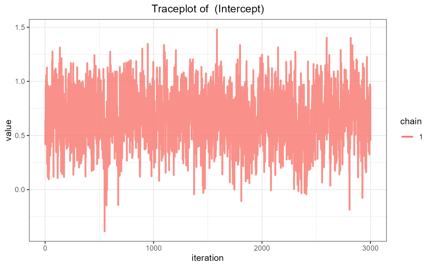
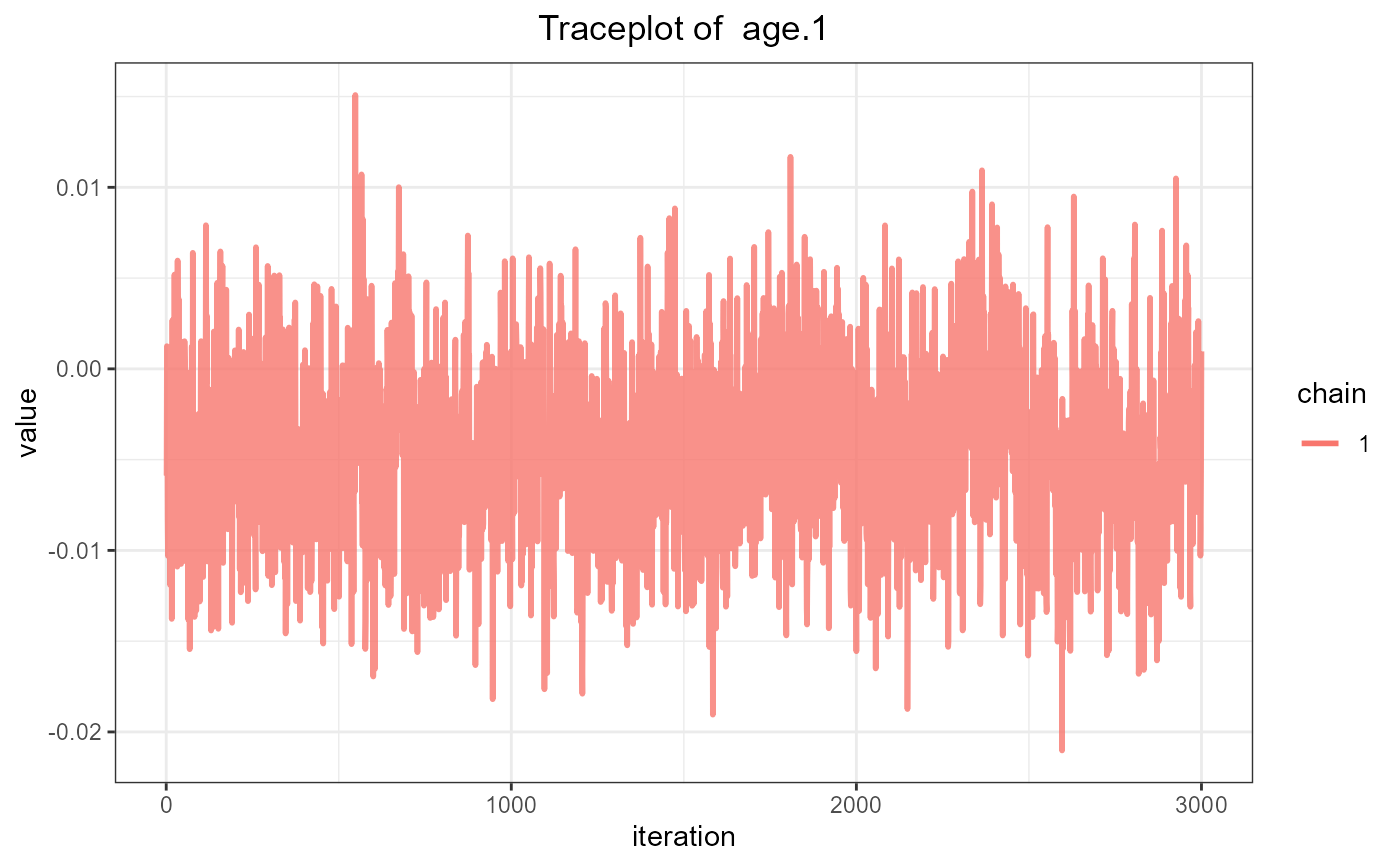
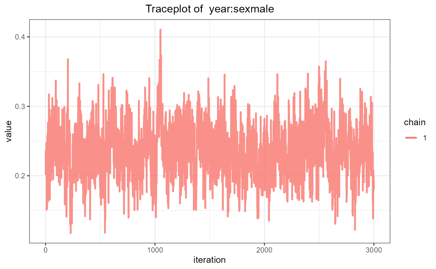
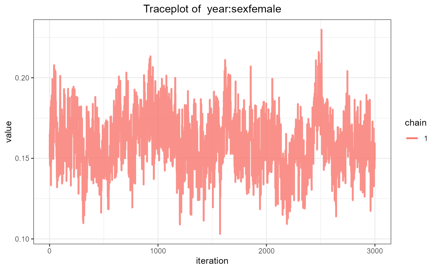
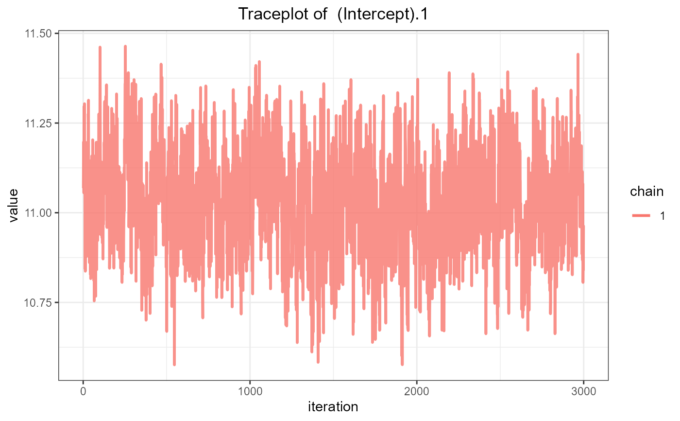
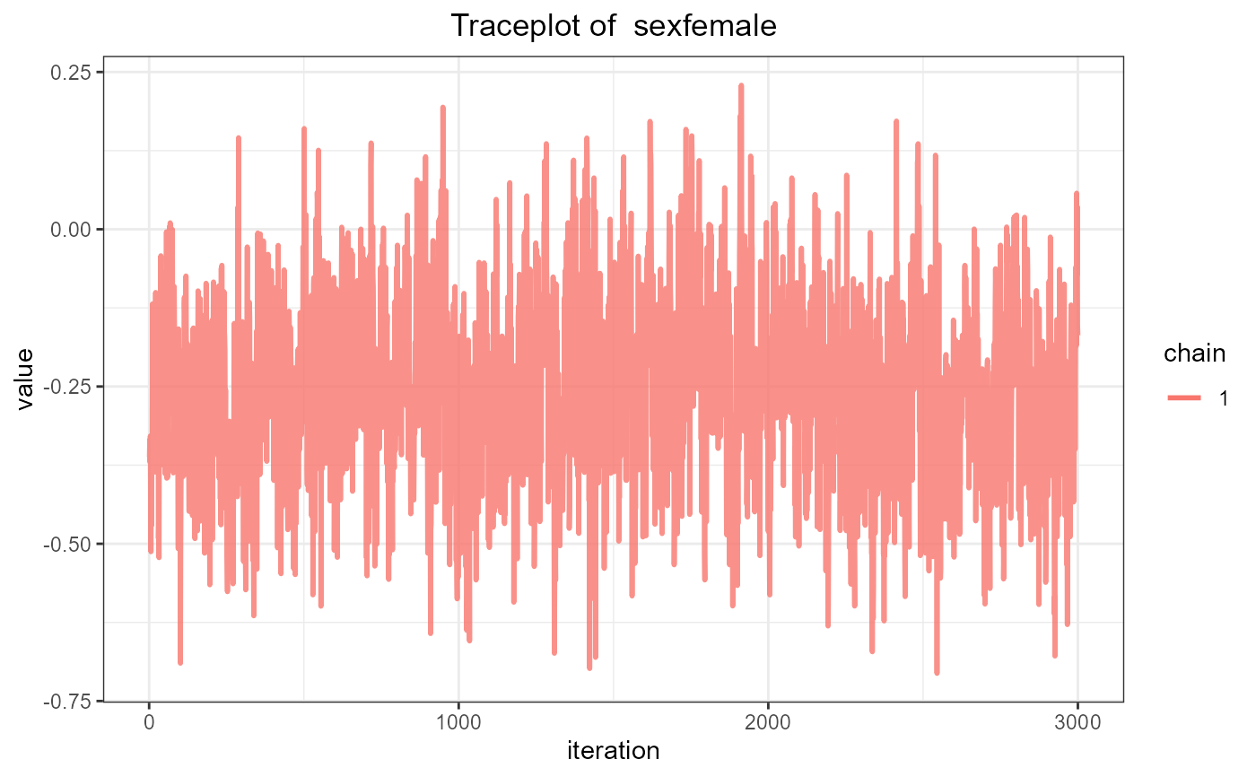
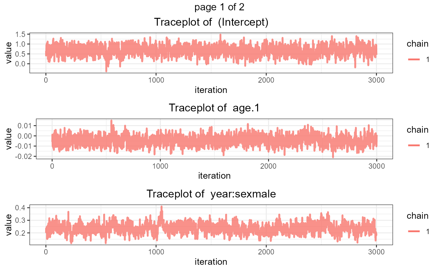
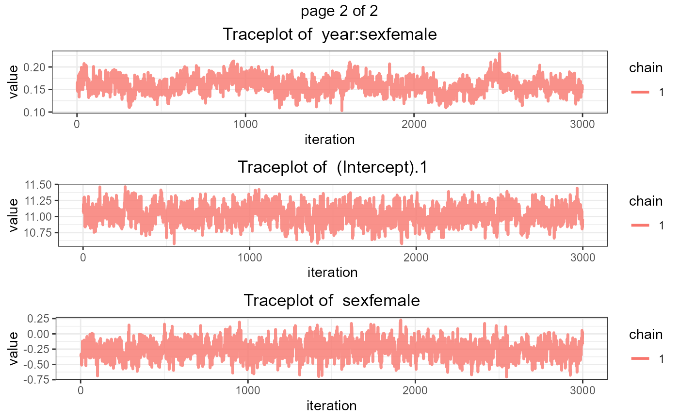
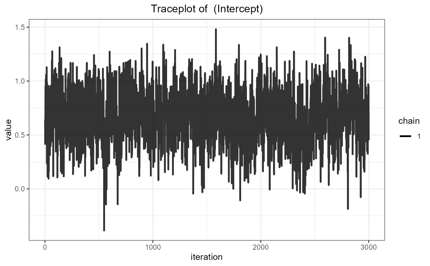
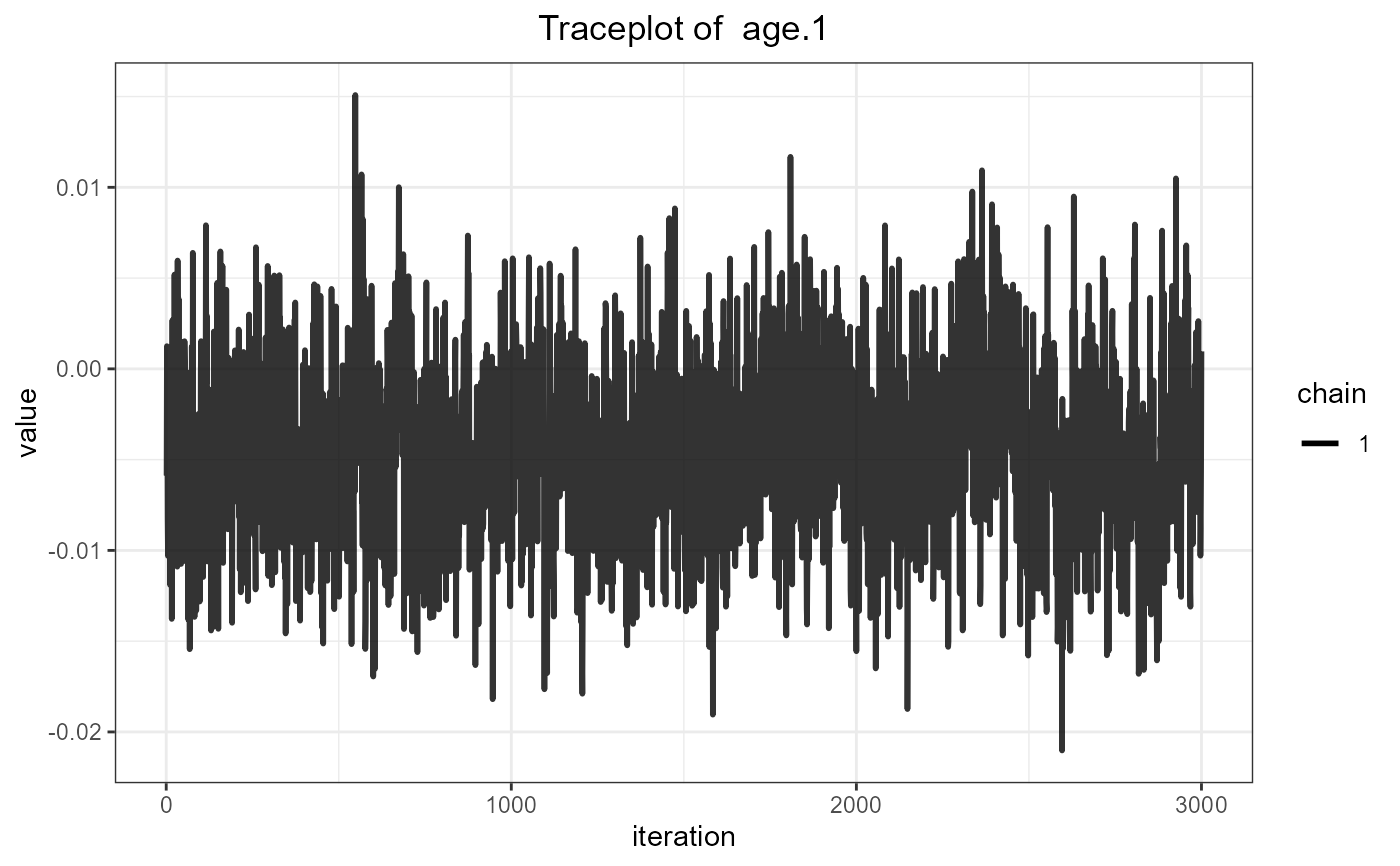
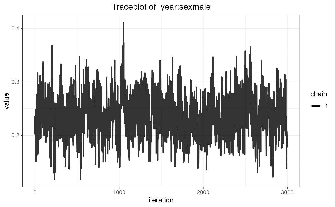
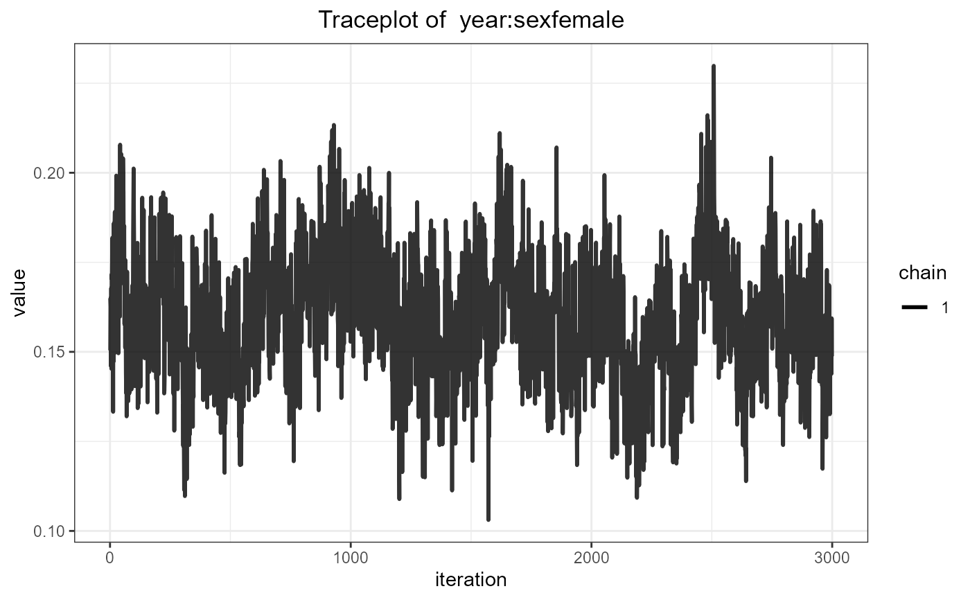
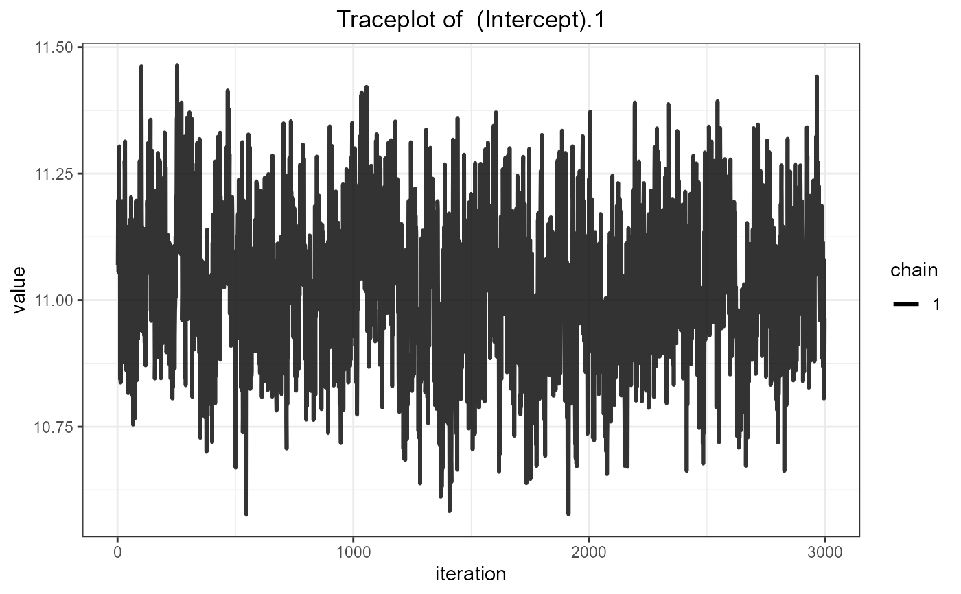
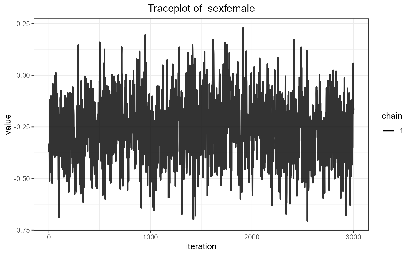
ggtraceplot()Plots the evolution of the estimated parameter vs. iterations in a fitted joint model using ggplot2.
gelman_diag()Calculates the potential scale reduction factor for the estimated parameters in a fitted joint model, together with the upper confidence limits.
densplot()Plots the density estimate for the estimated parameters in a fitted joint model.
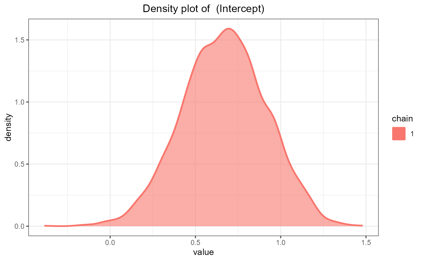
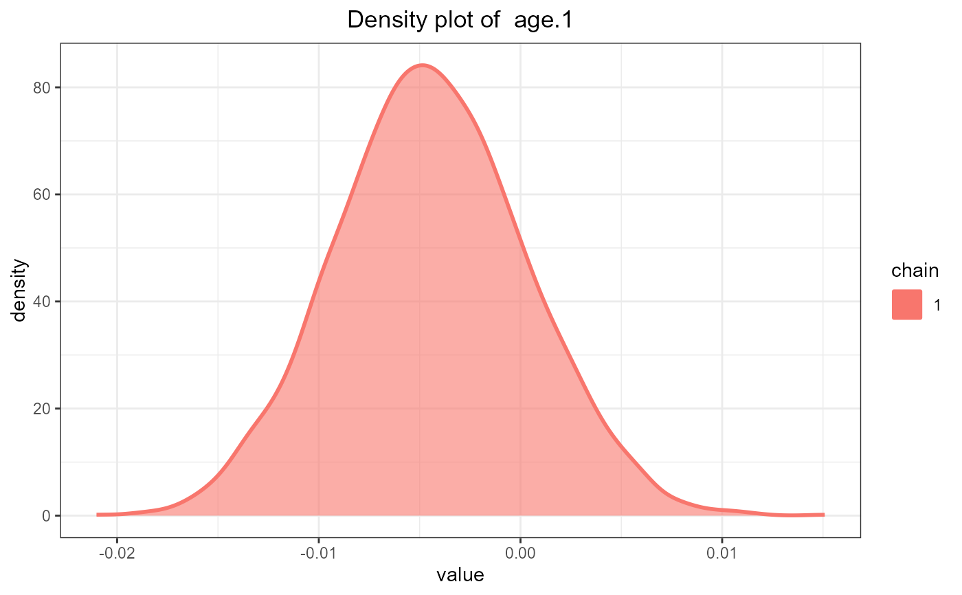
ggdensityplot()Plots the evolution of the estimated parameter vs. iterations in a fitted joint model using ggplot2.
cumuplot()Plots the evolution of the sample quantiles vs. iterations in a fitted joint model.
Author
Dimitris Rizopoulos d.rizopoulos@erasmusmc.nl
Examples
# \donttest{
# linear mixed model fits
fit_lme1 <- lme(log(serBilir) ~ year:sex + age,
random = ~ year | id, data = pbc2)
fit_lme2 <- lme(prothrombin ~ sex,
random = ~ year | id, data = pbc2)
# cox model fit
fit_cox <- coxph(Surv(years, status2) ~ age, data = pbc2.id)
# joint model fit
fit_jm <- jm(fit_cox, list(fit_lme1, fit_lme2), time_var = "year", n_chains = 1L)
# trace plot for the fixed effects in the linear mixed submodels
traceplot(fit_jm, parm = "betas")


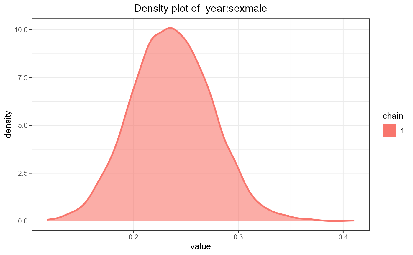
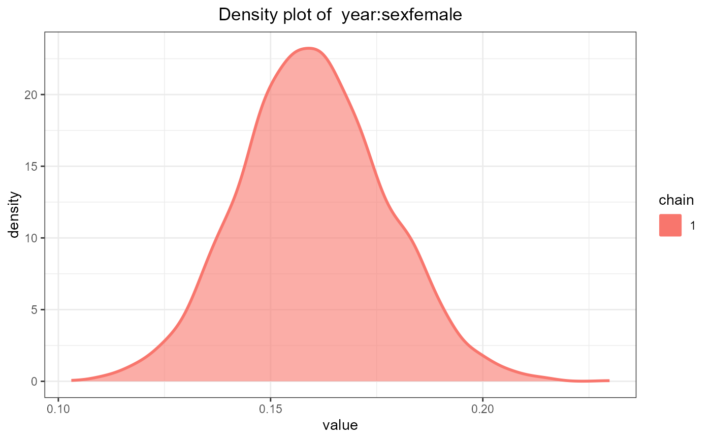
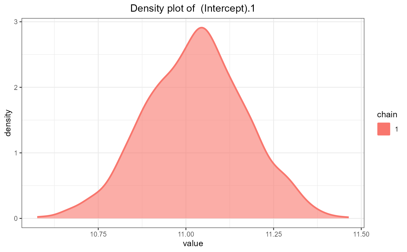
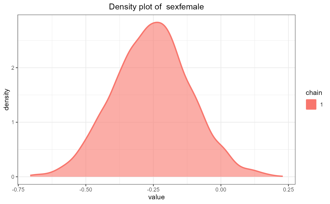
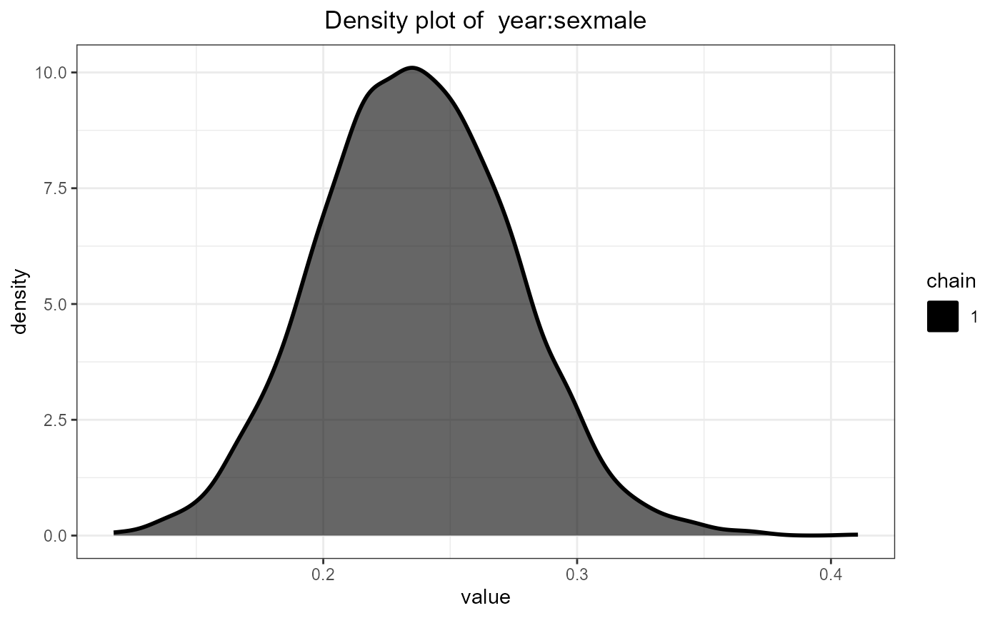
 # density plot for the fixed effects in the linear mixed submodels
densplot(fit_jm, parm = "betas")
# density plot for the fixed effects in the linear mixed submodels
densplot(fit_jm, parm = "betas")


 # cumulative quantile plot for the fixed effects in the linear mixed submodels
cumuplot(fit_jm, parm = "betas")
# cumulative quantile plot for the fixed effects in the linear mixed submodels
cumuplot(fit_jm, parm = "betas")

 # trace plot for the fixed effects in the linear mixed submodels
ggtraceplot(fit_jm, parm = "betas")
# trace plot for the fixed effects in the linear mixed submodels
ggtraceplot(fit_jm, parm = "betas")
 ggtraceplot(fit_jm, parm = "betas", grid = TRUE)
 ggtraceplot(fit_jm, parm = "betas", custom_theme = c('1' = 'black'))
 # trace plot for the fixed effects in the linear mixed submodels
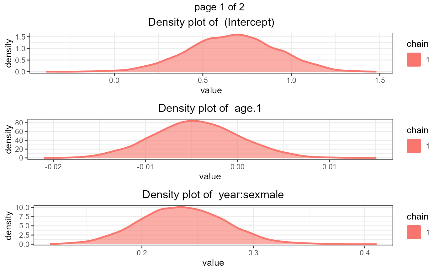
ggdensityplot(fit_jm, parm = "betas")
# trace plot for the fixed effects in the linear mixed submodels
ggdensityplot(fit_jm, parm = "betas")
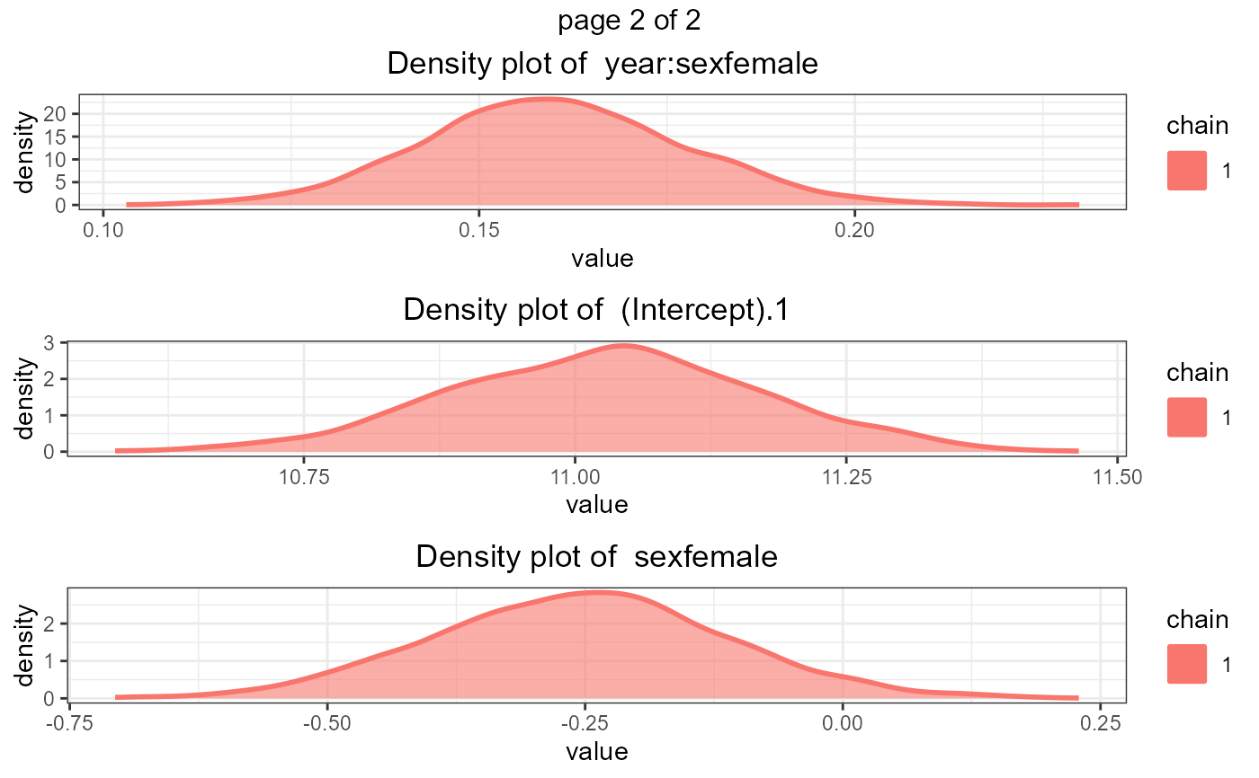
 ggdensityplot(fit_jm, parm = "betas", grid = TRUE)
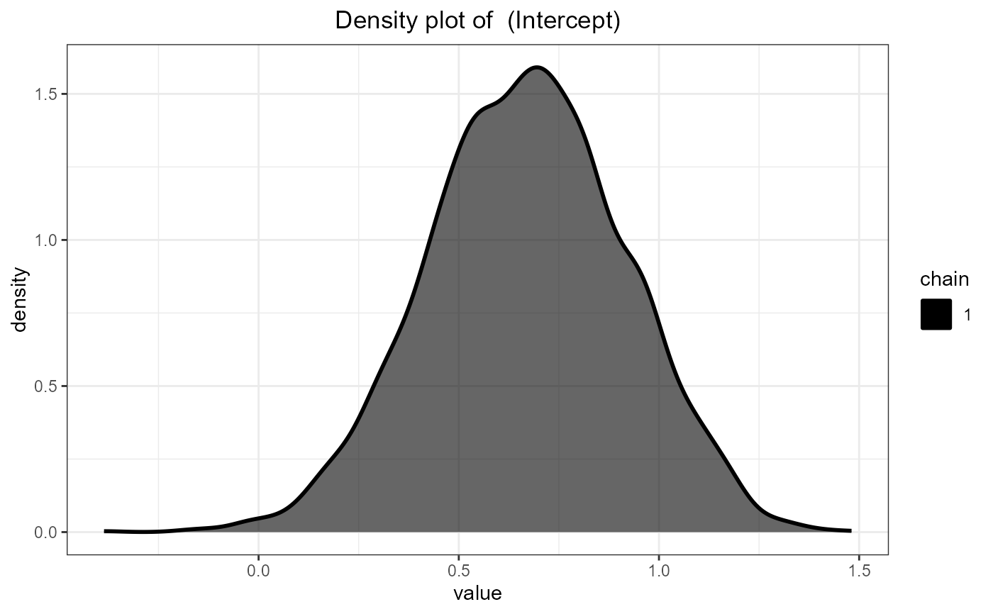
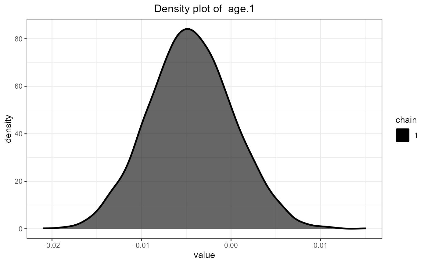
 ggdensityplot(fit_jm, parm = "betas", custom_theme = c('1' = 'black'))
 # }
# }