Predicted Values for Effects Plots
effectPlotData.RdCreates predicted values and their corresponding confidence interval for constructing an effects plot.
effectPlotData(object, newdata, level, ...)

# S3 method for class 'MixMod'
effectPlotData(object, newdata,
   level = 0.95, marginal = FALSE, CR_cohort_varname = NULL,
   direction = NULL, K = 200, seed = 1, sandwich = FALSE,
   ...)
Arguments
- object
an object inheriting from class
"MixMod".- newdata
a data frame base on which predictions will be calculated.
- level
a numeric scalar denoting the level of the confidence interval.
- marginal
logical; if
FALSEpredicted values are calculated for the "mean" subject (i.e., the one with random effects values equal to 0). WhenTRUEmarginal predicted values are calculated using functionmarginal_coefs.- CR_cohort_varname
a character string denoting the name of the cohort variable when a continuation ratio model is fitted.
- direction
the
directionargument ofcr_marg_probsneeds to be provided whenCR_cohort_varnameis notNULL.- K
numeric scalar denoting the number of Monte Carlo samples from the approximate posterior of the parameters; applicable only for zero-inflated models.
- seed
numerical scalar giving the seed to be used in the Monte Carlo scheme.
- sandwich
logical; if
TRUErobust/sandwich standard errors are used in the calculations.- ...
additional arguments passed to
marginal_coefs, e.g.,cores.
Details
The confidence interval is calculated based on a normal approximation.
Value
The data frame newdata with extra columns pred, low and upp.
See also
Examples
# \donttest{
# simulate some data
set.seed(123L)
n <- 500
K <- 15
t.max <- 25

betas <- c(-2.13, -0.25, 0.24, -0.05)
D <- matrix(0, 2, 2)
D[1:2, 1:2] <- c(0.48, -0.08, -0.08, 0.18)

times <- c(replicate(n, c(0, sort(runif(K-1, 0, t.max)))))
group <- sample(rep(0:1, each = n/2))
DF <- data.frame(year = times, group = factor(rep(group, each = K)))
X <- model.matrix(~ group * year, data = DF)
Z <- model.matrix(~ year, data = DF)

b <- cbind(rnorm(n, sd = sqrt(D[1, 1])), rnorm(n, sd = sqrt(D[2, 2])))
id <- rep(1:n, each = K)
eta.y <- as.vector(X %*% betas + rowSums(Z * b[id, ]))
DF$y <- rbinom(n * K, 1, plogis(eta.y))
DF$id <- factor(id)

################################################

# Fit a model
fm1 <- mixed_model(fixed = y ~ year * group, random = ~ year | id, data = DF,
                   family = binomial())

# An effects plot for the mean subject (i.e., with random effects equal to 0)
nDF <- with(DF, expand.grid(year = seq(min(year), max(year), length.out = 15),
    group = levels(group)))

plot_data <- effectPlotData(fm1, nDF)

require("lattice")
#> Loading required package: lattice
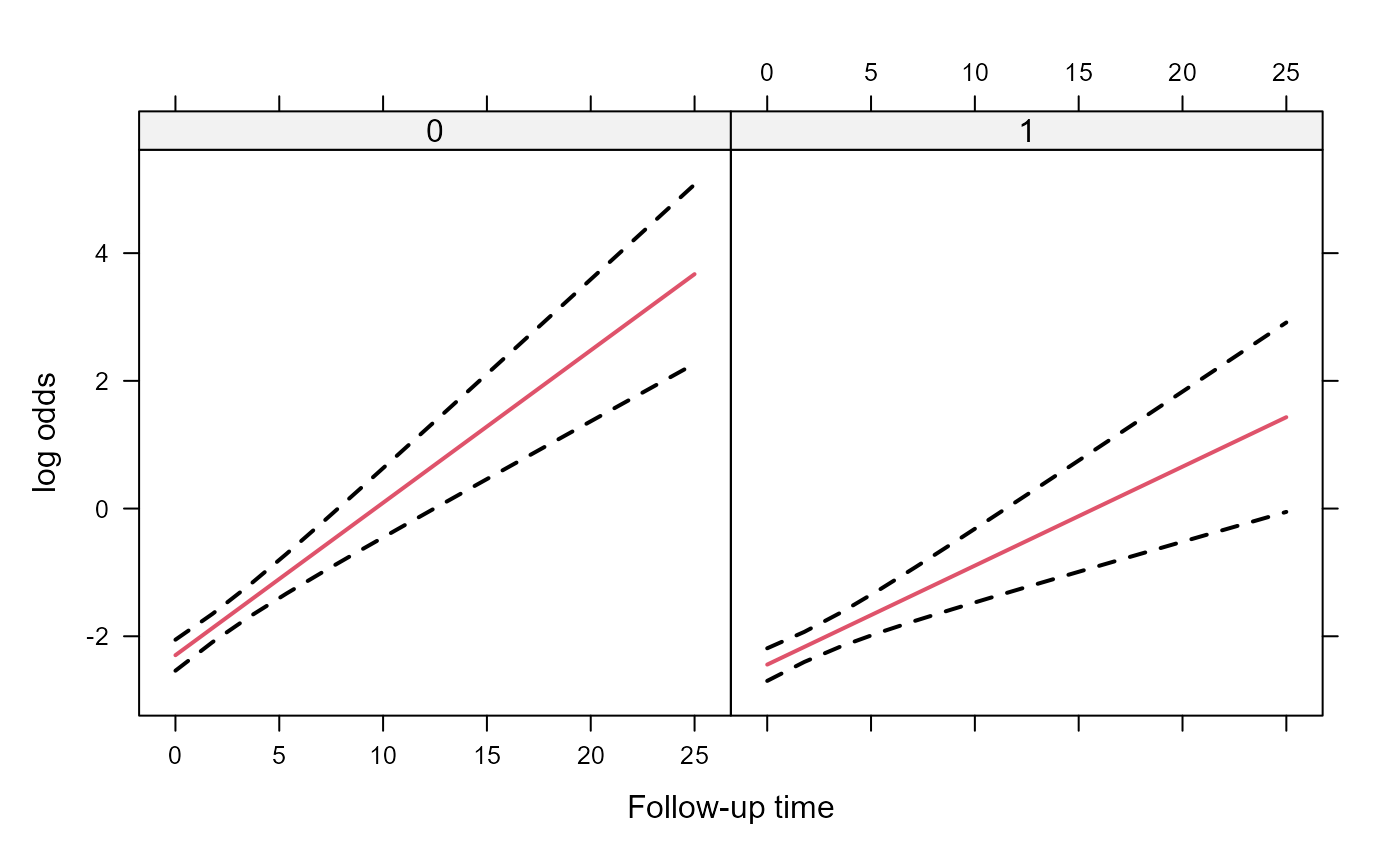
xyplot(pred + low + upp ~ year | group, data = plot_data,
       type = "l", lty = c(1, 2, 2), col = c(2, 1, 1), lwd = 2,
       xlab = "Follow-up time", ylab = "log odds")


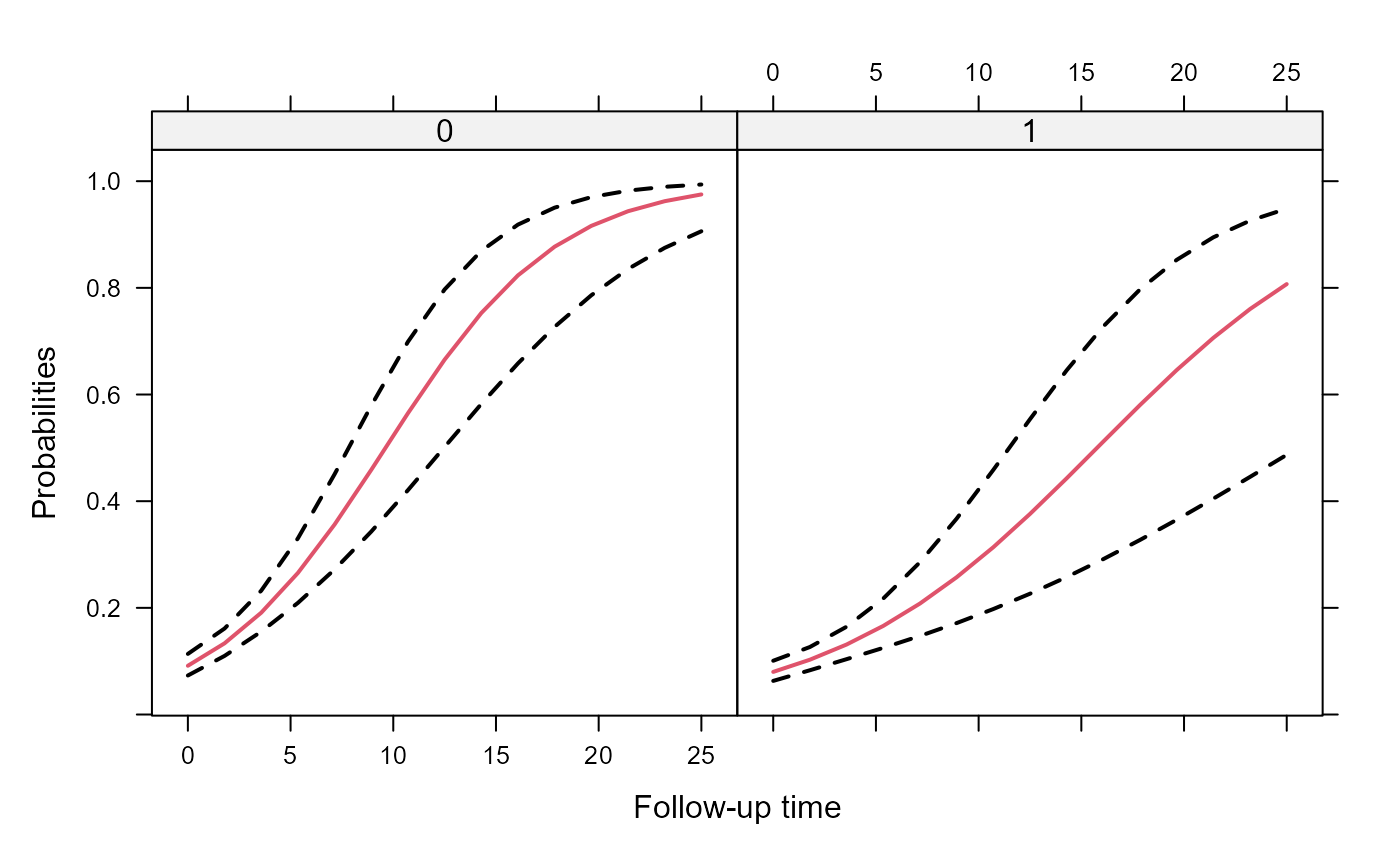
expit <- function (x) exp(x) / (1 + exp(x))
xyplot(expit(pred) + expit(low) + expit(upp) ~ year | group, data = plot_data,
       type = "l", lty = c(1, 2, 2), col = c(2, 1, 1), lwd = 2,
       xlab = "Follow-up time", ylab = "Probabilities")


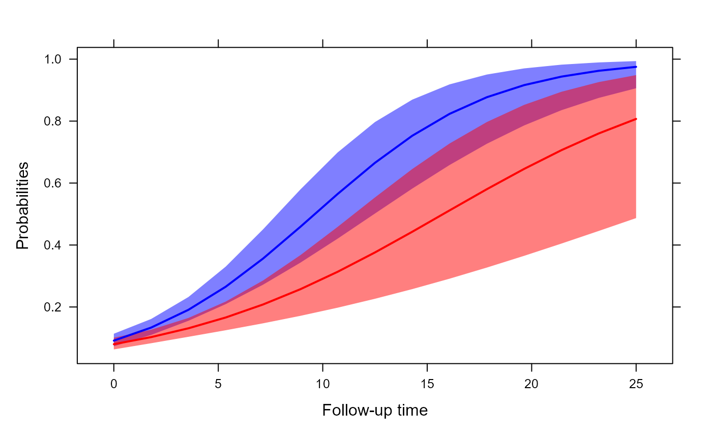
# we put the two groups in the same panel
my.panel.bands <- function(x, y, upper, lower, fill, col, subscripts, ..., font,
                           fontface) {
    upper <- upper[subscripts]
    lower <- lower[subscripts]
    panel.polygon(c(x, rev(x)), c(upper, rev(lower)), col = fill, border = FALSE, ...)
}

xyplot(expit(pred) ~ year, group = group, data = plot_data, upper = expit(plot_data$upp),
       low = expit(plot_data$low), type = "l", col = c("blue", "red"),
       fill = c("#0000FF80", "#FF000080"),
       panel = function (x, y, ...) {
           panel.superpose(x, y, panel.groups = my.panel.bands, ...)
           panel.xyplot(x, y, lwd = 2,  ...)
}, xlab = "Follow-up time", ylab = "Probabilities")


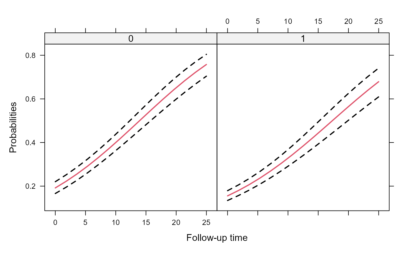
# An effects plots for the marginal probabilities
plot_data_m <- effectPlotData(fm1, nDF, marginal = TRUE, cores = 1L)

expit <- function (x) exp(x) / (1 + exp(x))
xyplot(expit(pred) + expit(low) + expit(upp) ~ year | group, data = plot_data_m,
       type = "l", lty = c(1, 2, 2), col = c(2, 1, 1), lwd = 2,
       xlab = "Follow-up time", ylab = "Probabilities")

# }
# }