Zero-Inflated and Two-Part Mixed Effects Models

Mixed Models with an Extra Zero Part

Function mixed_model() of GLMMadaptive can also be used to fit zero-inflated and two-part mixed effects models. For both types of models, a suitable family object needs to be specified as outlined in vignette("Custom_Models", package = "GLMMadaptive"), and also arguments zi_fixed and zi_random of mixed_model() come into play. In these arguments, the user can specify the fixed and random effects formulas of the logistic regression for the zero-part of the distribution of the outcome. We should note that the user has the option to leave zi_random set to NULL, in which case for the zero-part we have a logistic regression with only fixed effects and no random effects.

In addition, in the specification of the family object, and in order to better facilitate the internal computations, the user may specify the function score_eta_zi_fun that calculates the derivative of the log probability density function or the log probability mass function with respect to eta_zi that denotes the linear predictor of the logistic regression for the zero part. Here we provide three examples to illustrate how such models can be fitted.

Zero-Inflated Poisson Mixed Effects Model

We start our illustrations by showing how we can fit a zero-inflated Poisson mixed effects model. The specification of the required family object is already available in the package as the object returned by zi.poisson(). Currently, only the log link is allowed. First, we simulate longitudinal data from a zero-inflated negative binomial distribution:

set.seed(1234)
n <- 100 # number of subjects
K <- 8 # number of measurements per subject
t_max <- 5 # maximum follow-up time

# we construct a data frame with the design: 
# everyone has a baseline measurement, and then measurements at random follow-up times
DF <- data.frame(id = rep(seq_len(n), each = K),
                 time = c(replicate(n, c(0, sort(runif(K - 1, 0, t_max))))),
                 sex = rep(gl(2, n/2, labels = c("male", "female")), each = K))

# design matrices for the fixed and random effects non-zero part
X <- model.matrix(~ sex * time, data = DF)
Z <- model.matrix(~ 1, data = DF)
# design matrices for the fixed and random effects zero part
X_zi <- model.matrix(~ sex, data = DF)
Z_zi <- model.matrix(~ 1, data = DF)

betas <- c(1.5, 0.05, 0.05, -0.03) # fixed effects coefficients non-zero part
shape <- 2 # shape/size parameter of the negative binomial distribution
gammas <- c(-1.5, 0.5) # fixed effects coefficients zero part
D11 <- 0.5 # variance of random intercepts non-zero part
D22 <- 0.4 # variance of random intercepts zero part

# we simulate random effects
b <- cbind(rnorm(n, sd = sqrt(D11)), rnorm(n, sd = sqrt(D22)))
# linear predictor non-zero part
eta_y <- as.vector(X %*% betas + rowSums(Z * b[DF$id, 1, drop = FALSE]))
# linear predictor zero part
eta_zi <- as.vector(X_zi %*% gammas + rowSums(Z_zi * b[DF$id, 2, drop = FALSE]))
# we simulate negative binomial longitudinal data
DF$y <- rnbinom(n * K, size = shape, mu = exp(eta_y))
# we set the extra zeros
DF$y[as.logical(rbinom(n * K, size = 1, prob = plogis(eta_zi)))] <- 0

A zero-inflated Poisson mixed model with only fixed effects in the zero part is fitted with the following call to mixed_model():

fm1 <- mixed_model(y ~ sex * time, random = ~ 1 | id, data = DF,
                   family = zi.poisson(), zi_fixed = ~ sex)

fm1
#> 
#> Call:
#> mixed_model(fixed = y ~ sex * time, random = ~1 | id, data = DF, 
#>     family = zi.poisson(), zi_fixed = ~sex)
#> 
#> 
#> Model:
#>  family: zero-inflated poisson
#>  link: log 
#> 
#> Random effects covariance matrix:
#>                StdDev
#> (Intercept) 0.8272898
#> 
#> Fixed effects:
#>    (Intercept)      sexfemale           time sexfemale:time 
#>   1.5275644687   0.0173647260  -0.0040365383   0.0004326841 
#> 
#> Zero-part coefficients:
#> (Intercept)   sexfemale 
#>   -1.210597    0.498611 
#> 
#> log-Lik: -2223.937

As noted above, only the log link is currently available for the non-zero part and the logit link for the zero part. Hence, the estimated fixed effects for the two parts are interpreted accordingly. We extend fm1 by allowing also for random intercepts in the zero part. We should note that by default the random intercept of the non-zero part is correlated with the random intercept from the zero part:

fm2 <- update(fm1, zi_random = ~ 1 | id)

fm2
#> 
#> Call:
#> mixed_model(fixed = y ~ sex * time, random = ~1 | id, data = DF, 
#>     family = zi.poisson(), zi_fixed = ~sex, zi_random = ~1 | 
#>         id)
#> 
#> 
#> Model:
#>  family: zero-inflated poisson
#>  link: log 
#> 
#> Random effects covariance matrix:
#>                 StdDev    Corr
#> (Intercept)     0.7394        
#> zi_(Intercept)  0.6917 -0.6550
#> 
#> Fixed effects:
#>    (Intercept)      sexfemale           time sexfemale:time 
#>   1.5891884685  -0.0085650817  -0.0030156086   0.0002487272 
#> 
#> Zero-part coefficients:
#> (Intercept)   sexfemale 
#>   -1.112309    0.427672 
#> 
#> log-Lik: -2214.277

We test if we need the extra random effect using a likelihood ratio test:

anova(fm1, fm2)
#> 
#>         AIC     BIC  log.Lik   LRT df p.value
#> fm1 4461.87 4480.11 -2223.94                 
#> fm2 4446.55 4470.00 -2214.28 19.32  2   1e-04

The results suggest that the extra random effect improves the fit of the model.

Zero-Inflated Negative Binomial Mixed Effects Model

We continue with the same data, but we now take into account the potential over-dispersion in the data using a zero-inflated negative binomial model. To fit this mixed model we use an almost identical syntax to what we just did above - the only difference is that we now specify as family the zi.negative.binomial() object:

gm1 <- mixed_model(y ~ sex * time, random = ~ 1 | id, data = DF,
                   family = zi.negative.binomial(), zi_fixed = ~ sex)

gm1
#> 
#> Call:
#> mixed_model(fixed = y ~ sex * time, random = ~1 | id, data = DF, 
#>     family = zi.negative.binomial(), zi_fixed = ~sex)
#> 
#> 
#> Model:
#>  family: zero-inflated negative binomial
#>  link: log 
#> 
#> Random effects covariance matrix:
#>                StdDev
#> (Intercept) 0.8293515
#> 
#> Fixed effects:
#>    (Intercept)      sexfemale           time sexfemale:time 
#>    1.467900626    0.029416703    0.003005305   -0.006440699 
#> 
#> Zero-part coefficients:
#> (Intercept)   sexfemale 
#>  -1.5554713   0.5914944 
#> 
#> dispersion parameter:
#>  2.227075 
#> 
#> log-Lik: -1958.746

Similarly to fm1, in gm1 we specified only fixed effects for the logistic regression for the zero part. We now compare this model with the zero-inflated Poisson model that allowed for a random intercept in the zero part. The comparison can be done with the anova() method; because the two models are not nested, we set test = FALSE in the call to anova(), i.e.:

anova(gm1, fm2, test = FALSE)
#> 
#>         AIC     BIC  log.Lik df
#> gm1 3933.49 3954.33 -1958.75   
#> fm2 4446.55 4470.00 -2214.28  1

We observe that accounting for the over-dispersion seems to better improve the fit than including the random intercepts term in the zero part.

Two-Part Mixed Effects Model for Semi-Continuous Data

To further illustrate the flexibility provided by GLMMadaptive in allowing users to specify their own family objects with a specific log density function, we consider the setting of multivariate semi-continuous data. That is, continuous data with excess zeros. In the literature the class of two-part / hurdle mixed models has been proposed to analyze such data. These models specify a logistic regression for the dichotomous indicator that the outcome is zero or not, and a standard linear mixed model for the logarithmic transformation of the non-zero responses.

We start again by simulating some longitudinal data from this model:

set.seed(1234)
n <- 100 # number of subjects
K <- 8 # number of measurements per subject
t_max <- 5 # maximum follow-up time

# we construct a data frame with the design: 
# everyone has a baseline measurement, and then measurements at random follow-up times
DF <- data.frame(id = rep(seq_len(n), each = K),
                 time = c(replicate(n, c(0, sort(runif(K - 1, 0, t_max))))),
                 sex = rep(gl(2, n/2, labels = c("male", "female")), each = K))

# design matrices for the fixed and random effects non-zero part
X <- model.matrix(~ sex * time, data = DF)
Z <- model.matrix(~ time, data = DF)
# design matrices for the fixed and random effects zero part
X_zi <- model.matrix(~ sex, data = DF)
Z_zi <- model.matrix(~ 1, data = DF)

betas <- c(-2.13, -0.25, 0.24, -0.05) # fixed effects coefficients non-zero part
sigma <- 0.5 # standard deviation error terms non-zero part
gammas <- c(-1.5, 0.5) # fixed effects coefficients zero part
D11 <- 0.5 # variance of random intercepts non-zero part
D22 <- 0.1 # variance of random slopes non-zero part
D33 <- 0.4 # variance of random intercepts zero part

# we simulate random effects
b <- cbind(rnorm(n, sd = sqrt(D11)), rnorm(n, sd = sqrt(D22)), rnorm(n, sd = sqrt(D33)))
# linear predictor non-zero part
eta_y <- as.vector(X %*% betas + rowSums(Z * b[DF$id, 1:2, drop = FALSE]))
# linear predictor zero part
eta_zi <- as.vector(X_zi %*% gammas + rowSums(Z_zi * b[DF$id, 3, drop = FALSE]))
# we simulate log-normal longitudinal data
DF$y <- exp(rnorm(n * K, mean = eta_y, sd = sigma))
# we set the zeros from the logistic regression
DF$y[as.logical(rbinom(n * K, size = 1, prob = plogis(eta_zi)))] <- 0

To fit the two-part mixed model for log-normal data we can use the already build-in hurdle.lognormal() family object. However, just as an illustration, and to show that users can define their own family objects to be used in mixed_model(), we explain how exactly hurdle.lognormal() is specified. To define the family object: The minimal requirement is to specify the log_dens component and the link function; however, as also explained in the Custom Models vignette, the internal calculations will be faster and more stable if the user also specifies the score vector for the linear predictor of the non-zero part (function score_eta_fun()), the derivative of the log density with respect to phis (function score_phis_fun()), and because we have a model with a zero part, also the derivative of the log density with respect to the linear predictor of the zero part (function score_eta_zi_fun()). Finally, for being able to simulate from the model using the simulate() method, the function simulate() within the family object can also be specified. Hence, the family object for the two-part model is defined as:

hurdle.lognormal <- function () {
    stats <- make.link("identity")
    log_dens <- function (y, eta, mu_fun, phis, eta_zi) {
        sigma <- exp(phis)
        # binary indicator for y > 0
        ind <- y > 0
        # non-zero part
        eta <- as.matrix(eta)
        eta_zi <- as.matrix(eta_zi)
        out <- eta
        out[ind, ] <- plogis(eta_zi[ind, ], lower.tail = FALSE, log.p = TRUE) + 
            dnorm(x = log(y[ind]), mean = eta[ind, ], sd = sigma, log = TRUE)
        # zero part
        out[!ind, ] <- plogis(eta_zi[!ind, ], log.p = TRUE)
        attr(out, "mu_y") <- eta
        out
    }
    score_eta_fun <- function (y, mu, phis, eta_zi) {
        sigma <- exp(phis)
        # binary indicator for y > 0
        ind <- y > 0
        # non-zero part
        eta <- as.matrix(mu)
        out <- eta
        out[!ind, ] <- 0
        out[ind, ] <- (log(y[ind]) - eta[ind, ]) / sigma^2
        out
    }
    score_eta_zi_fun <- function (y, mu, phis, eta_zi) {
        ind <- y > 0
        probs <- plogis(as.matrix(eta_zi))
        out <- 1 - probs
        out[ind, ] <- - probs[ind, ]
        out
    }
    score_phis_fun <- function (y, mu, phis, eta_zi) {
        sigma <- exp(phis)
        # binary indicator for y > 0
        ind <- y > 0
        # non-zero part
        eta <- as.matrix(mu)
        out <- eta
        out[!ind, ] <- 0
        out[ind, ] <- - 1 + (log(y[ind]) - eta[ind, ])^2 / sigma^2
        out
    }
    simulate <- function (n, mu, phis, eta_zi) {
        y <- rlnorm(n = n, meanlog = mu, sdlog = exp(phis))
        y[as.logical(rbinom(n, 1, plogis(eta_zi)))] <- 0
        y
    }
    structure(list(family = "two-part log-normal", link = stats$name, 
                   linkfun = stats$linkfun, linkinv = stats$linkinv, log_dens = log_dens,
                   score_eta_fun = score_eta_fun, score_eta_zi_fun = score_eta_zi_fun,
                   score_phis_fun = score_phis_fun, simulate = simulate),
              class = "family")
}

Then to fit the model, we provide the user-defined family object in the family argument of mixed_model(), specifying also that we have one dispersion parameter in the family (i.e., n_phis = 1), and that in the zero part we only include fixed effects:

km1 <- mixed_model(y ~ sex * time, random = ~ 1 | id, data = DF, 
                  family = hurdle.lognormal(), n_phis = 1,
                  zi_fixed = ~ sex)

km1
#> 
#> Call:
#> mixed_model(fixed = y ~ sex * time, random = ~1 | id, data = DF, 
#>     family = hurdle.lognormal(), zi_fixed = ~sex, n_phis = 1)
#> 
#> 
#> Model:
#>  family: two-part log-normal
#>  link: identity 
#> 
#> Random effects covariance matrix:
#>                StdDev
#> (Intercept) 0.9609426
#> 
#> Fixed effects:
#>    (Intercept)      sexfemale           time sexfemale:time 
#>    -2.08122468    -0.24046281     0.22303981    -0.05686286 
#> 
#> Zero-part coefficients:
#> (Intercept)   sexfemale 
#>  -1.6034499   0.6713555 
#> 
#> phi parameters:
#>  -0.3348787 
#> 
#> log-Lik: -1214.208

The estimated standard deviation for the error terms is exp(phis) = 0.7 We extend the model by allowing for a random intercept in the zero-part, but using the || symbol in the random argument we specify the covariance matrix of the random effects is diagonal; hence, that the two random intercepts terms are uncorrelated:

km2 <- update(km1, random = ~ 1 || id, zi_random = ~ 1 | id)

km2
#> 
#> Call:
#> mixed_model(fixed = y ~ sex * time, random = ~1 || id, data = DF, 
#>     family = hurdle.lognormal(), zi_fixed = ~sex, zi_random = ~1 | 
#>         id, n_phis = 1)
#> 
#> 
#> Model:
#>  family: two-part log-normal
#>  link: identity 
#> 
#> Random effects covariance matrix:
#>                StdDev
#> (Intercept)    0.9609
#> zi_(Intercept) 0.6043
#> 
#> Fixed effects:
#>    (Intercept)      sexfemale           time sexfemale:time 
#>     -2.0811898     -0.2405682      0.2230215     -0.0568855 
#> 
#> Zero-part coefficients:
#> (Intercept)   sexfemale 
#>  -1.7160430   0.7096562 
#> 
#> phi parameters:
#>  -0.3349759 
#> 
#> log-Lik: -1210.313

For zero-inflated or hurdle models the marginal_coefs() functions provides the marginalized coefficients corresponding the average mixture response variable, i.e., \[(1 - \pi) \times E(Y),\] where \(\pi\) denotes the probability of being zero, and \(Y\) the response random variable for the non-zero part. For example, in the case of the hurdle log-normal family, we get the marginalized coefficients for \((1 - \pi) \times E\{\log(Y)\}\), e.g.,

marginal_coefs(km2)
#>    (Intercept)      sexfemale           time sexfemale:time 
#>        -1.7311         0.0626         0.1852        -0.0661

Finally, we show how the simulate() method can be used to perform a replication / posterior predictive check. In particular, in the following code we compare the empirical distribution function estimated in the observed data with estimates of the empirical distribution function obtained from simulated/replicated data from the model. In the call to simulate() below we also specify to account for the variability in the maximum likelihood estimates by setting acount_MLEs_var = TRUE:

par(mar = c(2.5, 2.5, 0, 0), mgp = c(1.1, 0.5, 0), cex.axis = 0.7, cex.lab = 0.8)
y <- DF$y
y[y > 0] <- log(y[y > 0])
x_vals <- seq(min(y), max(y), length.out = 500)
out <- simulate(km2, nsim = 30, acount_MLEs_var = TRUE)
ind <- out > sqrt(.Machine$double.eps)
out[ind] <- log(out[ind])
rep_y <- apply(out, 2, function (x, x_vals) ecdf(x)(x_vals), x_vals = x_vals)
matplot(x_vals, rep_y, type = "l", lty = 1, col = "lightgrey", 
        xlab = "Response Variable", ylab = "Empirical CDF")
lines(x_vals, ecdf(y)(x_vals))
legend("bottomright", c("log replicated data", "log observed data"), lty = 1, 
       col = c("lightgrey", "black"), bty = "n", cex = 0.8)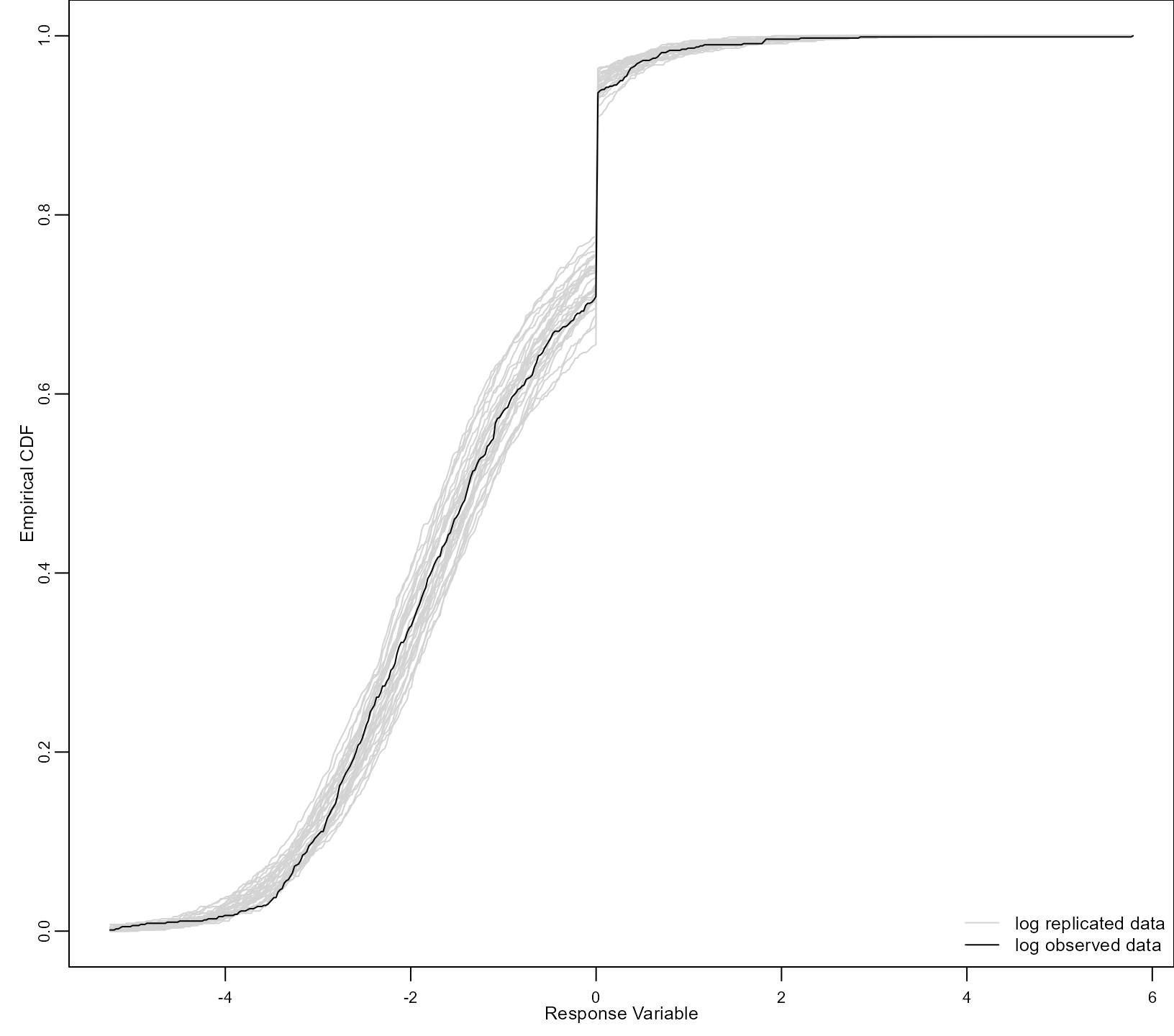

Two-Part/Hurdle Poisson Mixed Effects Model

An alternative modeling framework to account for high percentages of 0 in count data is hurdle models. These models are similar to the two-part model for semi-continuous data presented above. The difference is that for the positive part we have positive counts instead of a positive continuous outcome. For the positive counts, a truncated at zero Poisson or negative binomial distribution is typically used. Both hurdle Poisson and hurdle negative binomial mixed models can be fitted by mixed_model() using the family objects hurdle.poisson() and hurdle.negative.binomial, respectively.

To illustrate how these models are fitted, we simulate some longitudinal data from a hurdle negative binomial model using the code:

set.seed(123)
n <- 100 # number of subjects
K <- 8 # number of measurements per subject
t_max <- 5 # maximum follow-up time

# we construct a data frame with the design: 
# everyone has a baseline measurement, and then measurements at random follow-up times
DF <- data.frame(id = rep(seq_len(n), each = K),
                 time = c(replicate(n, c(0, sort(runif(K - 1, 0, t_max))))),
                 sex = rep(gl(2, n/2, labels = c("male", "female")), each = K))

# design matrices for the fixed and random effects non-zero part
X <- model.matrix(~ sex * time, data = DF)
Z <- model.matrix(~ time, data = DF)
# design matrices for the fixed and random effects zero part
X_zi <- model.matrix(~ sex, data = DF)
Z_zi <- model.matrix(~ 1, data = DF)

betas <- c(1.5, 0.05, 0.05, -0.03) # fixed effects coefficients non-zero part
shape <- 2 # shape/size parameter of the negative binomial distribution
gammas <- c(-1.5, 0.5) # fixed effects coefficients zero part
D11 <- 0.5 # variance of random intercepts non-zero part
D22 <- 0.1 # variance of random slopes non-zero part
D33 <- 0.4 # variance of random intercepts zero part

# we simulate random effects
b <- cbind(rnorm(n, sd = sqrt(D11)), rnorm(n, sd = sqrt(D22)), rnorm(n, sd = sqrt(D33)))
# linear predictor non-zero part
eta_y <- as.vector(X %*% betas + rowSums(Z * b[DF$id, 1:2, drop = FALSE]))
# linear predictor zero part
eta_zi <- as.vector(X_zi %*% gammas + rowSums(Z_zi * b[DF$id, 3, drop = FALSE]))
# we simulate truncated at zero negative binomial longitudinal data
lower <- pnbinom(0, mu = exp(eta_y), size = shape)
u <- runif(n * K, min = lower, max = 1)
DF$y <- qnbinom(u, mu = exp(eta_y), size = shape)
# we set the zeros from the logistic regression
DF$y[as.logical(rbinom(n * K, size = 1, prob = plogis(eta_zi)))] <- 0

The following code fits a hurdle Poisson mixed effects model. In the fixed-effects part for the positive counts we include the main effects of sex and time and their interaction, and in the random-effects for the positive counts random intercepts and random slopes. For the zero-part we only include a fixed-effects part, using argument zi_fixed, with sex as the predictor:

dm1 <- mixed_model(y ~ sex * time, random = ~ time | id, data = DF, 
                  family = hurdle.poisson(), zi_fixed = ~ sex)

dm1
#> 
#> Call:
#> mixed_model(fixed = y ~ sex * time, random = ~time | id, data = DF, 
#>     family = hurdle.poisson(), zi_fixed = ~sex)
#> 
#> 
#> Model:
#>  family: hurdle poisson
#>  link: log 
#> 
#> Random effects covariance matrix:
#>              StdDev    Corr
#> (Intercept)  0.8231        
#> time         0.3649 -0.3136
#> 
#> Fixed effects:
#>    (Intercept)      sexfemale           time sexfemale:time 
#>     1.52797499     0.08041345     0.08988228    -0.09127713 
#> 
#> Zero-part coefficients:
#> (Intercept)   sexfemale 
#>  -1.4178427   0.4857483 
#> 
#> log-Lik: -2802.3

Currently, only the log-link is implemented for the hurdle.poisson() family. The output is similar as in the case of the zero-inflated models. However, it has been noted that the fixed-effects coefficients for the positive counts part relate to the mean \(\mu\) of Poisson distribution that includes the zeros, not the mean for those who experience the event. The mean for those who experience more than one events is \(\mu / (1 - e^{-\mu})\). Hence, a \(\beta = 0.1\) cannot be interpreted as reflecting a \(e^\beta =\) 10% increase in the mean of the subjects who experience the events.

We extend model dm1 by also including a random intercept for the zero-part. As we have done above, this is achieved by specifying the zi_random argument, i.e.:

dm2 <- update(dm1, zi_random = ~ 1 | id)

dm2
#> 
#> Call:
#> mixed_model(fixed = y ~ sex * time, random = ~time | id, data = DF, 
#>     family = hurdle.poisson(), zi_fixed = ~sex, zi_random = ~1 | 
#>         id)
#> 
#> 
#> Model:
#>  family: hurdle poisson
#>  link: log 
#> 
#> Random effects covariance matrix:
#>                 StdDev    Corr        
#> (Intercept)     0.8226  (Intr)    time
#> time            0.3644 -0.3125        
#> zi_(Intercept)  0.6584 -0.0065  0.0636
#> 
#> Fixed effects:
#>    (Intercept)      sexfemale           time sexfemale:time 
#>     1.52792269     0.08389745     0.09206185    -0.08020395 
#> 
#> Zero-part coefficients:
#> (Intercept)   sexfemale 
#>  -1.5398382   0.5175922 
#> 
#> log-Lik: -2797.307

The likelihood ratio test between the two models is computed with the anova() method:

anova(dm1, dm2)
#> 
#>         AIC     BIC  log.Lik  LRT df p.value
#> dm1 5622.60 5646.05 -2802.30                
#> dm2 5618.61 5649.88 -2797.31 9.99  3  0.0187

The result indicates that the extra random effect for the zero-part improves the fit of the model.

Two-Part/Hurdle Negative Binomial Mixed Effects Model

We continue our illustration of hurdle models by fitting the hurdle negative binomial mixed model. The only change from the previous syntax we used is the name of the family object, namely, we use now hurdle.negative.binomial(). The code below fits exactly the same model as model dm1 above, but using now the negative binomial distribution for the positive counts:

hm1 <- mixed_model(y ~ sex * time, random = ~ time | id, data = DF, 
                  family = hurdle.negative.binomial(), zi_fixed = ~ sex)

hm1
#> 
#> Call:
#> mixed_model(fixed = y ~ sex * time, random = ~time | id, data = DF, 
#>     family = hurdle.negative.binomial(), zi_fixed = ~sex)
#> 
#> 
#> Model:
#>  family: hurdle negative binomial
#>  link: log 
#> 
#> Random effects covariance matrix:
#>              StdDev    Corr
#> (Intercept)  0.7305        
#> time         0.3249 -0.1170
#> 
#> Fixed effects:
#>    (Intercept)      sexfemale           time sexfemale:time 
#>     1.48250218     0.07508276     0.10249953    -0.08978082 
#> 
#> Zero-part coefficients:
#> (Intercept)   sexfemale 
#>  -1.4178427   0.4857483 
#> 
#> phi parameters:
#>  0.6778918 
#> 
#> log-Lik: -2181.468

Also for the hurdle.negative.binomial() family only the log-link is implemented. The structure of the output is identical to what we had for the hurdle Poisson model. Again we should note that the fixed-effects coefficients for the positive part have an interpretation for the mean of the entire distribution, not only for the positive counts.

We update again the fitted model hm1 by including a random intercept for the zero-part:

hm2 <- update(hm1, zi_random = ~ 1 | id)

hm2
#> 
#> Call:
#> mixed_model(fixed = y ~ sex * time, random = ~time | id, data = DF, 
#>     family = hurdle.negative.binomial(), zi_fixed = ~sex, zi_random = ~1 | 
#>         id)
#> 
#> 
#> Model:
#>  family: hurdle negative binomial
#>  link: log 
#> 
#> Random effects covariance matrix:
#>                 StdDev    Corr        
#> (Intercept)     0.7315  (Intr)    time
#> time            0.3258 -0.1155        
#> zi_(Intercept)  0.6598 -0.0517  0.1412
#> 
#> Fixed effects:
#>    (Intercept)      sexfemale           time sexfemale:time 
#>     1.47627667     0.07040678     0.10535938    -0.08613120 
#> 
#> Zero-part coefficients:
#> (Intercept)   sexfemale 
#>  -1.5420047   0.5197229 
#> 
#> phi parameters:
#>  0.6759598 
#> 
#> log-Lik: -2176.312