Generalized Linear Mixed Effects Models

Fits generalized linear mixed effects models under maximum likelihood using adaptive Gaussian quadrature.

mixed_model(fixed, random, data, family, weights = NULL,
  na.action = na.exclude, zi_fixed = NULL, zi_random = NULL, 
  penalized = FALSE, n_phis = NULL, initial_values = NULL, 
  control = list(), ...)

Arguments

fixed

a formula for the fixed-effects part of the model, including the outcome.

random

a formula for the random-effects part of the model. This should only contain the right-hand side part, e.g., ~ time | id, where time is a variable, and id the grouping factor. When the symbol || is used in the definition of this argument (instead of |), then the covariance matrix of the random effects is assumed to be diagonal.

data

a data.frame containing the variables required in fixed and random.

family

a family object specifying the type of the repeatedly measured response variable, e.g., binomial() or poisson(). The function also allows for user-defined family objects, but with specific extra components; see the example is negative.binomial for more details. Contrary to the standard practice in model fitting R functions with a family argument (e.g., glm) in which the default family is gaussian(), in mixed_model() no default is provided. If the users wish to fit a mixed model for a Gaussian outcome, this could be done with function lme() from the nlme package or function lmer() from the lme4 package.

weights

a numeric vector of weights. These are simple multipliers on the log-likelihood contributions of each group/cluster, i.e., we presume that there are multiple replicates of each group/cluster denoted by the weights. The length of `weights` need to be equal to the number of independent groups/clusters in the data.

na.action

what to do with missing values in data.

zi_fixed, zi_random

formulas for the fixed and random effects of the zero inflated part.

penalized

logical or a list. If logical and equal to FALSE, then no penalty is used. If logical and equal to TRUE, for the fixed effects a Student's-t penalty/prior with mean 0, scale equal to 1 and 3 degrees of freedom is used. If a list, then it is expected to have the components pen_mu, pen_sigma and pen_df, denoting the mean, scale and degrees of freedom of the Student's-t penalty/prior for the fixed effects.

n_phis

a numeric scalar; in case the family corresponds to a distribution that has extra (dispersion/shape) parameters, you need to specify how many extra parameters are needed.

initial_values

a list of initial values. This can have up to three components, namely,

betas: a numeric vector of fixed effects. This can also be family object. In this case initial values for the fixed effects will be calculated by using glm to the data ignoring the correlations in the repeated measurements. For example, for a negative binomial response outcome, we could set betas = poisson().
D: a numeric matrix denoting the covariance matrix of the random effects.
phis: a numeric vector for the extra (dispersion/shape) parameters.

control

a list with the following components:

iter_EM: numeric scalar denoting the number of EM iterations; default is 30.
iter_qN_outer: numeric scalar denoting the number of outer iterations during the quasi-Newton phase; default is 15. In each outer iteration the locations of the quadrature points are updated.
iter_qN: numeric scalar denoting the starting number of iterations for the quasi-Newton; default is 10.
iter_qN_incr: numeric scalar denoting the increment in iter_qN for each outer iteration; default is 10.
optimizer: character string denoting the optimizer to be used; available options are "optim" (default), "nlminb" and "optimParallel", the last option implemented in the optimParallel package.
optim_method: character string denoting the type of optim algorithm to be used when optimizer = "optim"; default is the BFGS algorithm.
parscale_betas: the control argument parscale of optim for the fixed-effects; default is 0.1.
parscale_D: the control argument parscale of optim for the unique element of the covariance matrix of the random effects; default is 0.01.
parscale_phis: the control argument parscale of optim for the extra (dispersion/shape) parameters; default is 0.01.
tol1, tol2, tol3: numeric scalars controlling tolerances for declaring convergence; tol1 and tol2 are for checking convergence in successive parameter values; tol3 is similar to reltop of optim; default values are 1e-03, 1e-04, and 1e-08, respectively.
numeric_deriv: character string denoting the type of numerical derivatives to be used. Options are "fd" for forward differences, and cd for central difference; default is "fd".
nAGQ: numeric scalar denoting the number of quadrature points; default is 11 when the number of random effects is one or two, and 7 otherwise.
update_GH_every: numeric scalar denoting every how many iterations to update the quadrature points during the EM-phase; default is 10.
max_coef_value: numeric scalar denoting the maximum allowable value for the fixed effects coefficients during the optimization; default is 10.
max_phis_value: numeric scalar denoting the maximum allowable value for the shape/dispersion parameter of the negative binomial distribution during the optimization; default is exp(10).
verbose: logical; print information during the optimization phase; default is FALSE.

...

arguments passed to control.

Details

General: The mixed_model() function fits mixed effects models in which the integrals over the random effects in the definition of the marginal log-likelihood cannot be solved analytically and need to be approximated. The function works under the assumption of normally distributed random effects with mean zero and variance-covariance matrix \(D\). These integrals are approximated numerically using an adaptive Gauss-Hermite quadrature rule. Using the control argument nAGQ, the user can specify the number of quadrature points used in the approximation.

User-defined family: The user can define its own family object; for an example, see the help page of negative.binomial.

Optimization: A hybrid approach is used, starting with iter_EM iterations and unless convergence was achieved it continuous with a direct optimization of the log-likelihood using function optim and the algorithm specified by optim_method. For stability and speed, the derivative of the log-likelihood with respect to the parameters are internally programmed.

Value

An object of class "MixMod" with components:

coefficients: a numeric vector with the estimated fixed effects.
phis: a numeric vector with the estimated extra parameters.
D: a numeric matrix denoting the estimated covariance matrix of the random effects.
post_modes: a numeric matrix with the empirical Bayes estimates of the random effects.
post_vars: a list of numeric matrices with the posterior variances of the random effects.
logLik: a numeric scalar denoting the log-likelihood value at the end of the optimization procedure.
Hessian: a numeric matrix denoting the Hessian matrix at the end of the optimization procedure.
converged: a logical indicating whether convergence was attained.
data: a copy of the data argument.
id: a copy of the grouping variable from data.
id_name: a character string with the name of the grouping variable.
Terms: a list with two terms components, termsX derived from the fixed argument, and termsZ derived from the random argument.
model_frames: a list with two model.frame components, mfX derived from the fixed argument, and mfZ derived from the random argument.
control: a copy of the (user-specific) control argument.
Funs: a list of functions used in the optimization procedure.
family: a copy of the family argument.
call: the matched call.

Author

Dimitris Rizopoulos d.rizopoulos@erasmusmc.nl

Examples

# simulate some data
set.seed(123L)
n <- 200
K <- 15
t.max <- 25

betas <- c(-2.13, -0.25, 0.24, -0.05)
D <- matrix(0, 2, 2)
D[1:2, 1:2] <- c(0.48, -0.08, -0.08, 0.18)

times <- c(replicate(n, c(0, sort(runif(K-1, 0, t.max)))))
group <- sample(rep(0:1, each = n/2))
DF <- data.frame(year = times, group = factor(rep(group, each = K)))
X <- model.matrix(~ group * year, data = DF)
Z <- model.matrix(~ year, data = DF)

b <- cbind(rnorm(n, sd = sqrt(D[1, 1])), rnorm(n, sd = sqrt(D[2, 2])))
id <- rep(1:n, each = K)
eta.y <- as.vector(X %*% betas + rowSums(Z * b[id, ]))
DF$y <- rbinom(n * K, 1, plogis(eta.y))
DF$id <- factor(id)

################################################

fm1 <- mixed_model(fixed = y ~ year * group, random = ~ 1 | id, data = DF,
                   family = binomial())

# fixed effects
fixef(fm1)
#> (Intercept)        year      group1 year:group1 
#> -2.51135823  0.23304276 -0.88784195 -0.05174851 

# random effects
head(ranef(fm1))
#>   (Intercept)
#> 1   0.2428149
#> 2   2.1943191
#> 3   1.2898486
#> 4  -1.2667384
#> 5  -0.7294567
#> 6   3.1614903

# detailed output
summary(fm1)
#> 
#> Call:
#> mixed_model(fixed = y ~ year * group, random = ~1 | id, data = DF, 
#>     family = binomial())
#> 
#> Data Descriptives:
#> Number of Observations: 3000
#> Number of Groups: 200 
#> 
#> Model:
#>  family: binomial
#>  link: logit 
#> 
#> Fit statistics:
#>    log.Lik      AIC      BIC
#>  -1225.973 2461.947 2478.438
#> 
#> Random effects covariance matrix:
#>               StdDev
#> (Intercept) 2.851543
#> 
#> Fixed effects:
#>             Estimate Std.Err z-value   p-value
#> (Intercept)  -2.5114  0.3430 -7.3216   < 1e-04
#> year          0.2330  0.0155 15.0812   < 1e-04
#> group1       -0.8878  0.4816 -1.8437 0.0652272
#> year:group1  -0.0517  0.0195 -2.6534 0.0079694
#> 
#> Integration:
#> method: adaptive Gauss-Hermite quadrature rule
#> quadrature points: 11
#> 
#> Optimization:
#> method: hybrid EM and quasi-Newton
#> converged: TRUE 

# fitted values for the 'mean subject', i.e., with
# random effects values equal to 0
head(fitted(fm1, type = "mean_subject"))
#>          1          2          3          4          5          6 
#> 0.03232047 0.03944053 0.10950605 0.17572685 0.20676636 0.20921567 

# fitted values for the conditioning on the estimated random effects
head(fitted(fm1, type = "subject_specific"))
#>          1          2          3          4          5          6 
#> 0.04084042 0.04974091 0.13552321 0.21370151 0.24941898 0.25221291 

##############
# \donttest{
fm2 <- mixed_model(fixed = y ~ year, random = ~ 1 | id, data = DF,
                   family = binomial())

# likelihood ratio test between the two models
anova(fm2, fm1)
#> 
#>         AIC     BIC  log.Lik  LRT df p.value
#> fm2 2477.04 2486.94 -1235.52                
#> fm1 2461.95 2478.44 -1225.97 19.1  2   1e-04
#> 

# the same hypothesis but with a Wald test
anova(fm1, L = rbind(c(0, 0, 1, 0), c(0, 0, 0, 1)))
#> 
#> Marginal Wald Tests Table
#> 
#> User-defined contrasts matrix:
#>  (Intr) year group1 yr:gr1
#>       0    0      1      0
#>       0    0      0      1
#> 
#>     Chisq df Pr(>|Chi|)
#>   18.7743  2      1e-04
#> 

##############

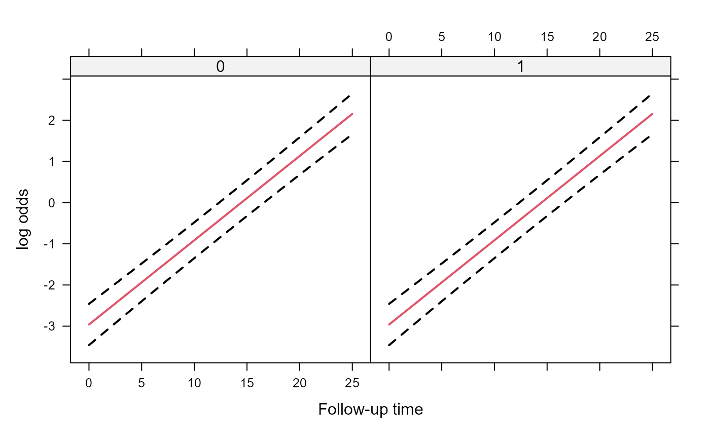
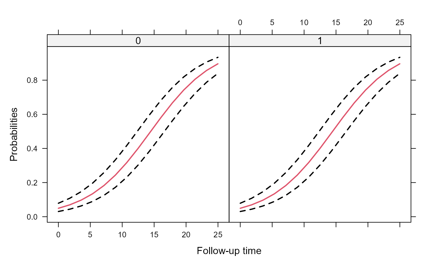
# An effects plot for the mean subject (i.e., with random effects equal to 0)
nDF <- with(DF, expand.grid(year = seq(min(year), max(year), length.out = 15),
    group = levels(group)))
    
plot_data <- effectPlotData(fm2, nDF)

require("lattice")
xyplot(pred + low + upp ~ year | group, data = plot_data,
       type = "l", lty = c(1, 2, 2), col = c(2, 1, 1), lwd = 2,
       xlab = "Follow-up time", ylab = "log odds")


expit <- function (x) exp(x) / (1 + exp(x))
xyplot(expit(pred) + expit(low) + expit(upp) ~ year | group, data = plot_data,
       type = "l", lty = c(1, 2, 2), col = c(2, 1, 1), lwd = 2,
       xlab = "Follow-up time", ylab = "Probabilities")


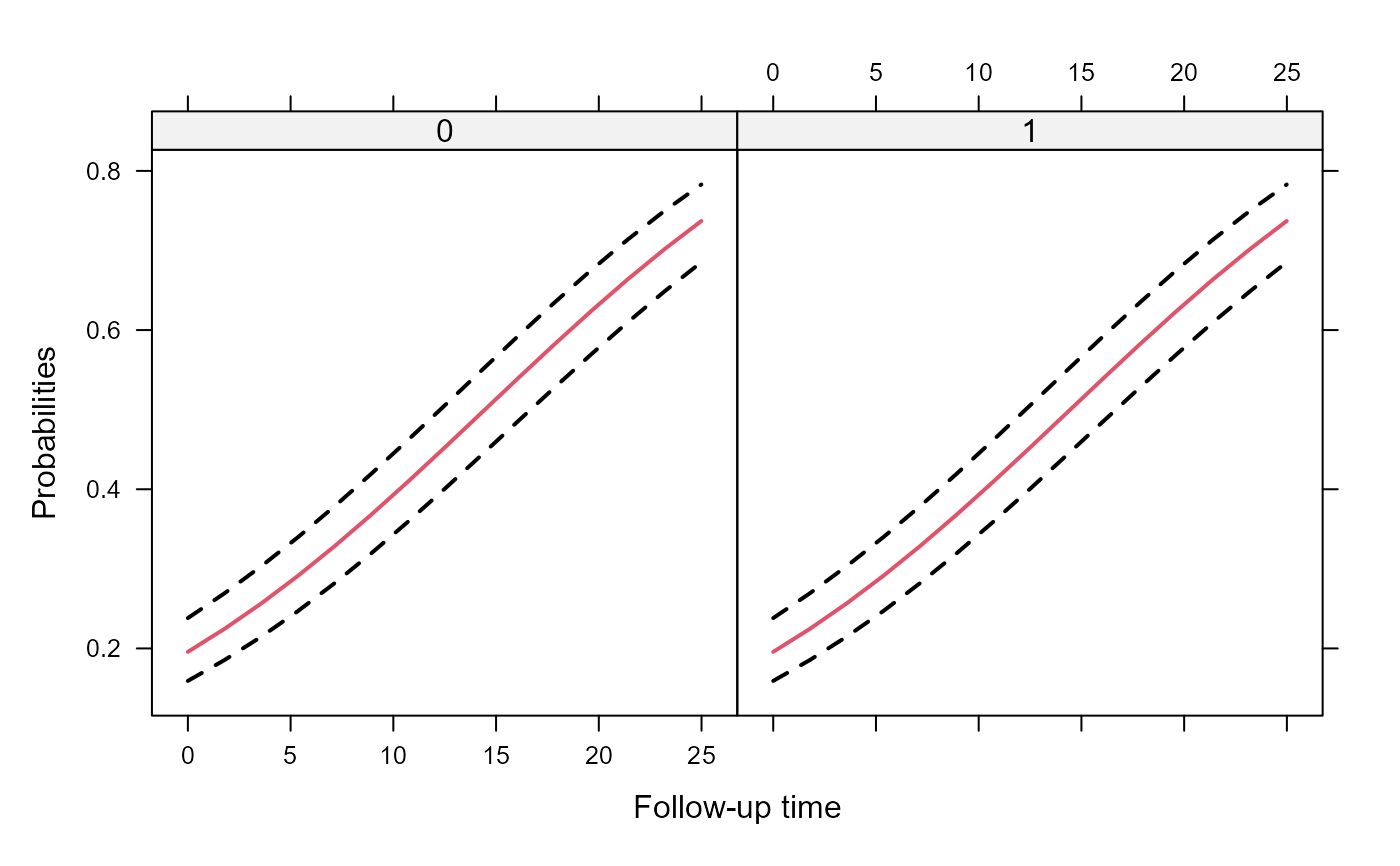
# An effects plots for the marginal probabilities
plot_data_m <- effectPlotData(fm2, nDF, marginal = TRUE, cores = 1L)

expit <- function (x) exp(x) / (1 + exp(x))
xyplot(expit(pred) + expit(low) + expit(upp) ~ year | group, data = plot_data_m,
       type = "l", lty = c(1, 2, 2), col = c(2, 1, 1), lwd = 2,
       xlab = "Follow-up time", ylab = "Probabilities")


##############

# include random slopes
fm1_slp <- update(fm1, random = ~ year | id)

# increase the number of quadrature points to 15
fm1_slp_q15 <- update(fm1_slp, nAGQ = 15)

# a diagonal covariance matrix for the random effects
fm1_slp_diag <- update(fm1, random = ~ year || id)

anova(fm1_slp_diag, fm1_slp)
#> 
#>                  AIC     BIC  log.Lik  LRT df p.value
#> fm1_slp_diag 2112.08 2131.87 -1050.04                
#> fm1_slp      2113.83 2136.91 -1049.91 0.25  1  0.6141
#> 
# }

Arguments

Details

Value

Author

See also

Examples