• To avoid over-treatment, men with low grade prostate cancer are advised active surveillance

• Cancer progression is tracked via:
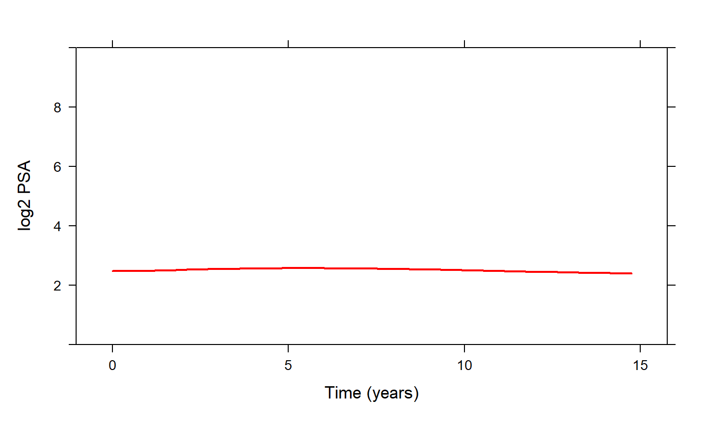
  • Prostate-specific antigen measurements
  • Digital rectal examination
  • MRI
  • Biopsies

• Treatment is advised when cancer progression is observed
  • typically via biopsies when Gleason Score \(\geq 7\)

• Two dimensions
  • Number of biopsies
  • Delay in finding progression

• Delay: We want to find progression asap

• Number of biopsies: high burden
  • painful, cause complications, expensive

• Annual Biopsies
  • focus on minimizing delay
  • many unnecessary biopsies for patients who progress slow

• Less Frequent Biopsies - PRIAS
  • every 3 years or
  • annually if PSA doubling time < 10 (try to find faster progressions)
  • still unnecessary biopsies for patients who progress slow

• unnecessary biopsies \(\Rightarrow\) Low compliance
  • effectiveness of AS is compromised

• Scheduling based on individualized risk predictions
  • Progression rate is not only different between patients but also dynamically changes over time for the same patient

• Risk predictions based upon
  • All available PSA (ng/mL) measurements
  • All available DRE (T1c / above T1c) measurements
  • Time and results of previous biopsies

• In steps:
  • How the longitudinal PSA & DRE are related to Gleason reclassification?
  • How to combine previous PSA & DRE measurements and biopsies to predict reclassification?
  • When to plan the next biopsy?

• To answer these questions we need to link
  • the time to Gleason reclassification (survival outcome)
  • the PSA measurements (longitudinal continuous outcome)
  • the DRE measurements (longitudinal binary outcome)

• Biomarkers are endogenous time-varying covariates
  • their future path depends on previous events
  • standard time-varying Cox model not appropriate

• We need some notation
  • \(T_i^*\) the true reclassification time
  • \(T_i^L\) last biopsy time point Gleason Score was \(< 7\)
  • \(T_i^R\) first biopsy time point Gleason Score was \(\geq 7\)
  • \(T_i^R = \infty\) for patients who haven’t been reclassified yet
  • \(\mathbf y_{i1}\) vector of longitudinal PSA measurements
  • \(\mathcal Y_{i1}(t) = \{y_{i1}(s), 0 \leq s < t\}\)
  • \(\mathbf y_{i2}\) vector of longitudinal DRE measurements
  • \(\mathcal Y_{i2}(t) = \{y_{i2}(s), 0 \leq s < t\}\)

\[\left \{ \begin{array}{ccl} h_i(t) & = & h_0(t) \exp \{\mathbf \gamma^\top \mathbf w_i + \alpha_1 {\color{red} \eta_{i1}(t)} + \alpha_2 {\color{blue} \eta_{i2}(t)}\}\\&&\\ y_{i1}(t) & = & {\color{red} \eta_{i1}(t)} + \varepsilon_i(t)\\ & = & \mathbf x_{i1}^\top(t) \mathbf \beta_1 + \mathbf z_{i1}^\top(t) \mathbf b_{i1} + \varepsilon_i(t)\\&&\\ \log\frac{\Pr\{y_{i2}(t) = 1\}}{1 - \Pr\{y_{i2}(t) = 1\}} & = & {\color{blue} \eta_{i2}(t)}\\ & = & \mathbf x_{i2}^\top(t) \mathbf \beta_2 + \mathbf z_{i2}^\top(t) \mathbf b_{i2}\\&&\\ \mathbf \{b_{i1}, b_{i2}\} \sim \mathcal N(\mathbf 0, \mathbf D), & & \varepsilon_i(t) \sim \mathcal N(0, \sigma^2) \end{array} \right.\]

• The longitudinal and survival outcomes are jointly modeled \[\begin{eqnarray} p(y_{i1}, y_{i2}, T_i^L, T_i^R) & = & \int p(y_{i1} \mid {\color{red} b_{i1}}) \; p(y_{i2} \mid {\color{red} b_{i2}}) \times \\ && \quad \quad \left\{S(T_i^L \mid {\color{red} b_i}) - S(T_i^R \mid {\color{red} b_i})\right\} p({\color{red} b_i}) \; d{\color{red} b_i}\\ \end{eqnarray}\]
  
  • the random effects \({\color{red} b_i}\) explain the interdependencies

• PSA velocity

  • fast increasing PSA indicative of progression

  
  

  \[h_i(t) = h_0(t) \exp \{\mathbf \gamma^\top \mathbf w_i + \alpha_1 {\color{red} \eta_{i1}(t)} + \alpha_2 {\color{blue} \eta_{i1}'(t)} + \alpha_3 {\color{red} \eta_{i2}(t)}\}\]
  where \({\color{blue} \eta_{i1}'(t)} = \frac{d}{dt} \eta_{i1}(t)\)

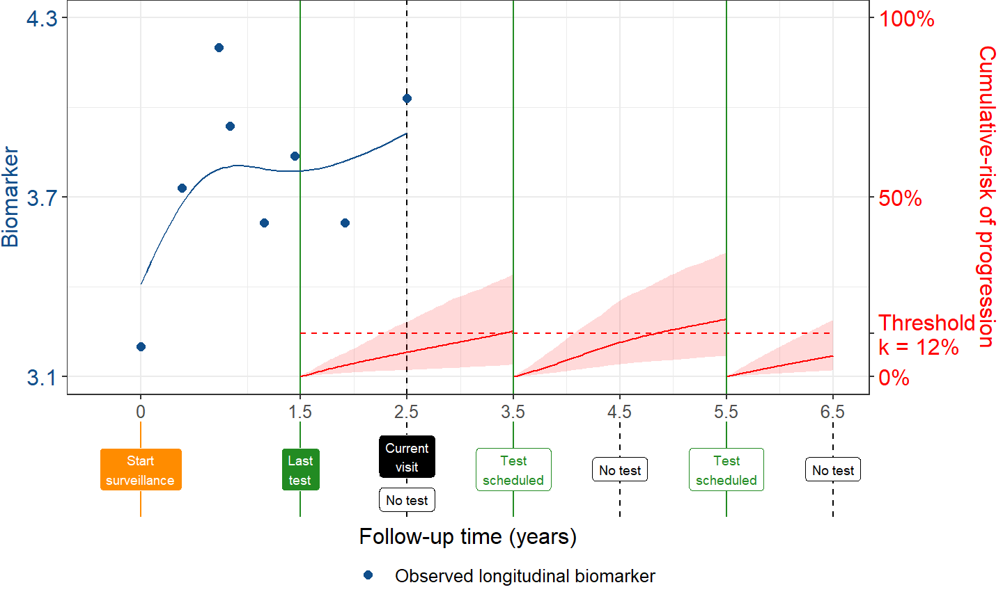
• Using the fitted joint model we can calculate the cumulative risk of progression \[\pi_j(u \mid t, v) = \Pr \bigl \{ T_j^* \leq u \mid T_j^* \geq t, \mathcal Y_{j1}(v), \mathcal Y_{j2}(v) \bigr \}\]

• \(t\) time of last biopsy
• \(v\) time of current visit, \(v \geq t\)
• \(u\) future time, \(u \geq t\)
• \(\mathcal Y_{j1}(v)\) & \(\mathcal Y_{j2}(v)\) available PSA & DRE measurements up to current visit

• Patients come back every 6 months for PSA & DRE measurements
  • at these occasions we want to decide for a biopsy

• In general, we consider decisions at a fixed schedule \[\begin{array}{l} s_1, \ldots, s_N\\ s_1 = v\\ s_N = h \end{array}\]

• Simple decision rule: We do a biopsy at \(s_n\) if
  
  \[\pi(s_n \mid t_n, v) \geq \kappa_n\]
• where
  • \(\kappa_n\) a threshold at \(s_n\)
  • \(t_n\) time of last biopsy before \(s_n\)

• The key question is

• We consider two relevant quantities
  • the number of biopsies
  • the delay in finding progression

• For different thresholds \(\kappa_n\) we would obtain different number of biopsies and different delays…

• For a specific threshold \(\kappa^*\) we can calculate
  • how many times a biopsy will be performed in the future

• The times when biopsies are performed \[t_n = \left\{ \begin{array}{l} t_{n-1} : \pi_j(s_n \mid t_{n - 1}, v) < \kappa^*\\\\ s_n : \pi_j(s_n \mid t_{n - 1}, v) \geq \kappa^*\\ \end{array} \right.\]

• The expected number of biopsies will be \[\mathcal N_j(\kappa^*) = \sum_{n = 1}^N \mbox{I}\{\pi_j(s_n \mid t_n, v) \geq \kappa^*\} \times \{1 - \pi_j(t_{n-1} \mid t, v)\}\]

• For a specific threshold \(\kappa^*\) we can calculate
  • the expected delay \[\begin{array}{lcl} \mathcal D_j(\kappa^*) & = & \sum\limits_{n = 1}^N \bigl \{ t_n - E(T_j^* \mid t_{n-1} \leq T_j^* \leq t_n) \bigr \} \times\\&&\\ && \quad \quad \Pr \bigl \{ t_{n-1} \leq T_j^* \leq t_n \mid T_j^* > t, \mathcal Y_{j1}(v), \mathcal Y_{j2}(v) \bigr \} \end{array}\]

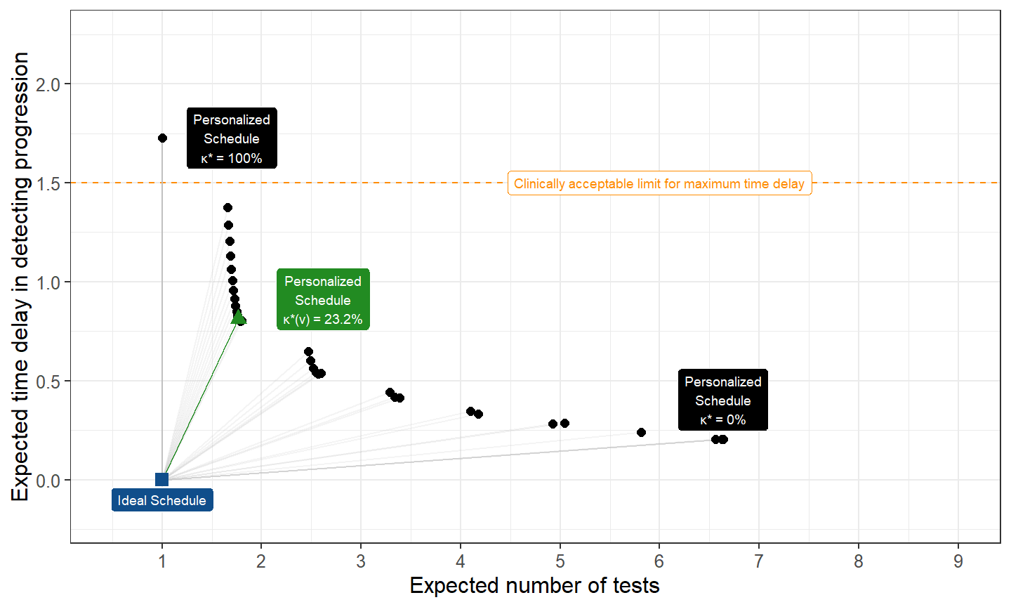
• For different \(\kappa\)’s we construct the two-dimensional space of expected number of biopsies and expected delays

• If we consider that the delay & the number of biopsies are equally important
  • we can select the \(\kappa_n\) that is closest to the optimal schedule \[{\color{red} \kappa_n^{opt}} = \mbox{argmin}_{\kappa} \sqrt{ \bigl \{ \mathcal N_j(\kappa) - 1 \bigr \}^2 + \mathcal D_j(\kappa)^2}\]

• Othrewise,
  • we may also select a clinically acceptable delay, and
  • select \({\color{red} \kappa_n^{opt}}\) the \(\kappa\) that minimizes the expected number of biopsies

• Calibration
  • calculation of expected delay and number of biopsies require a well-calibrated model

• Schedules become more personalized the better biomarkers distinguish patients
  • consider more biomarkers, e.g., for postate cancer MRI

• Paper available at:
  • Biometrics
  • Medical Decision Making
  • Statistics in Medicine

• Software: available in JMbayes on CRAN & GitHub
  • https://cran.r-project.org/package=JMbayes
  • https://github.com/drizopoulos/JMbayes

• Online shiny app available at https://emcbiostatistics.shinyapps.io/prias_biopsy_recommender/